Spectral Analytical Filter¶

This block performs multiplication, in spectral space, by an analytical function depending only on the total wavenumber. The block is self-adjoint, so the block’s multiply() and multiplyAD() methods are identical.

The two typical use-cases are for frequency filters in The ProcessPerts Application or for Horizontal Localization Mode in a general variational application (implemented in SABER as a dirac test in the The ErrorCovarianceToolbox Application).

In both cases, this block should appear above (in the list of saber outer blocks in the yaml configuration) a transformation to spectral space (for instance the Spectral To Gauss block) as it operates on fieldSets in the frequency domain. In typical cases, a spectral representation of a fieldSet will be transformed from a Regular Gaussian grid (see Gaussian Grids for more information). In this case, the default maximum waveband in the spectral representation will be \(2N-1\) where \(N\) is the Gaussian Number of the regular gaussian grid.

We refer the reader to [EMenard12] for an explanation of how these filters relate to isotropic convolutions.

Frequency Filter Mode¶

This block can be used as a bandpass filter (applied to each vertical level) on fieldSets that have been transformed into frequency space. Several filter profiles for attenuating waveband coefficients are available:

triangle (trapeziod for special cases)
boxcar (rectangle)
gaussian

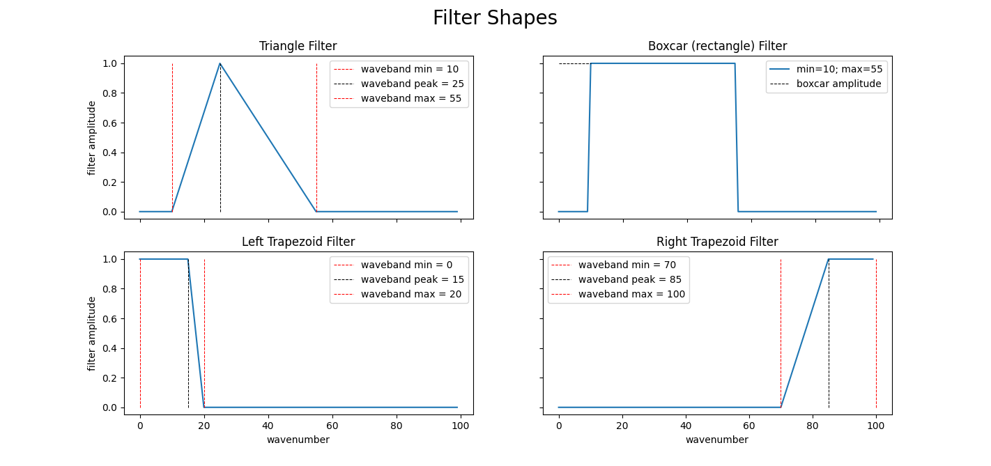
To use the triangle filter profile, the user provides a waveband min, waveband peak, and waveband max to specify the filter profile. If the lowest waveband (\(n = 0\)) is the waveband min or the maximum waveband in your truncation is the waveband max; then, the filter will create a trapezoidal profile and set the attenuation to 1 between the waveband end-point and the waveband peak. To use the boxcar profile, the user provides a waveband min, waveband max, and waveband amplitude. See Filter Shapes and yaml examples below for more information.

../../../_images/figure_filter_shapes.png

Fig. 8 Triangle and boxcar filter profiles (top). Special trapeziod cases of the triangle profile (below).¶

Example yaml: Triangle/Trapeziod filter¶

To use a triangle filter profile, choose waveband fitler for shape in the filter function settings, and select waveband parameters. If waveband min is zero, the filter profile will be a left trapeziod and if waveband max is equal to the maximum number kept in the spectral transformation the profile will have the right trapeziod profile (see Filter Shapes).

saber outer blocks:
  - (*** inner blocks ***)
  - saber block name: spectral analytical filter
    function:
      shape: waveband filter        # "waveband filter" selects the triangle profile
      waveband min: wb_min          # (int) minimum waveband
      waveband peak: wb_peak        # (int) peak waveband
      waveband max: wb_max          # (int) maximum waveband
    preserving variance: true       # (bool) set to 'true' in filtering mode
    active variables: *vars         # variables to be filtered
  -(*** outer blocks ***)

Note

For more information on the preserving variance parameter, see the Main idea (waveband filter mode) section of the ProcessPerts documentation.

Example yaml: Boxcar filter¶

saber outer blocks:
  - (*** inner blocks ***)
  - saber block name: spectral analytical filter
    function:
      shape: boxcar            # "boxcar" selects the rectangle profile
      waveband min: wb_min     # (int) minimum waveband of box
      waveband max: wb_max     # (int) maximum waveband of box
      waveband amplitude: 1.0  # amplitude of box
    preserving variance: true  # (bool) set to 'true' in filtering mode
    active variables: *vars    # variables to be filtered
  -(*** outer blocks ***)

Example yaml: Gaussian filter¶

saber outer blocks:
- (...)
- saber block name: spectral analytical filter
  normalize filter variance: false  # Optional. Default is true (for localization)
  function:
    shape: gaussian                 # Optional. Default is gaussian.
    horizontal daley length: 2000e3
- (...)

The parameter normalize filter variance decides whether the analytical function should be normalized to act as a localization function (so should be set to false in filter mode).

Horizontal Localization Mode¶

This block can be used for horizontal localization, relying on the fact that convolution on the physical space is equivalent to multiplication on the spectral space. In this use-case, only the gaussian filter profile (function) is recommended.

To model convolution by a Gaussian localization function \(f(d)\) in physical space (where \(d\) is the great circle separation distance), we multiply by a Gaussian localization function \(\widehat{f}(n)\) in spectral space (where \(n\) is the total wavenumber). If the physical space Gaussian is given by

\[\begin{split}f(d) &= \exp\biggl(-\frac{d^2}{2 L^2}\biggr)\\ \text{Or equivalently }f(\lambda) &= \exp\biggl(-\frac{\lambda^2}{2 \sigma_{\lambda}^2}\biggr)\end{split}\]

where \(L\) is the horizontal localization length, \(d = \lambda R\), \(R\) is the Earth radius and \(\sigma_\lambda = L / R\), then the associated Gaussian in spectral space is given by:

\[\widehat{f}(n) = C\exp\biggl(-\frac{n^2}{2\sigma_n^2}\biggr)\]

where \(\sigma_n = 1/ \sigma_\lambda = R / L\) and \(C\) is some normalization constant.

The normalization constant \(C\) is computed by ensuring the total variance of the localization function in spectral space is 1.

Example yaml (localization)¶

- saber block name: spectral analytical filter
  function:
    horizontal daley length: 2000e3

Here, the localization is modeled as a Gaussian with Daley length specified from the yaml, in meters. For a Gaussian function, the Daley length \(\sqrt{-f(0) / f''(0)}\) is parameter \(L\) in the equations above (see for instance [PBD08]).

Since the spectral analytical localization is a (self-adjoint) outer block, it is actually applied twice in a multiplication by the associated localization or covariance matrix. The block accounts for this in the definition of the Daley length \(L\), so that the full correlation model (with the outer block applied twice) has a Daley length \(L\).