Correlated Observation Error Covariance with Diffusion

The diffusion-based correlated R operator in UFO applies the oops::Diffusion capability similar to how it is implemented in SABER by the Explicit Diffusion block. Both operators use a forward stepping finite-difference method to propagate error covariances to nearby locations (see [WCMP21] for more details of the implementation, though the paper discusses implicit diffusion the calibration process discussed in the reference is implemented by this operator).

When initialized, the UFO operator constructs a mesh from the observation locations read from the observations’ ioda::ObsSpace (see figure below). Diffusion will occur along edges that connect observation locations.

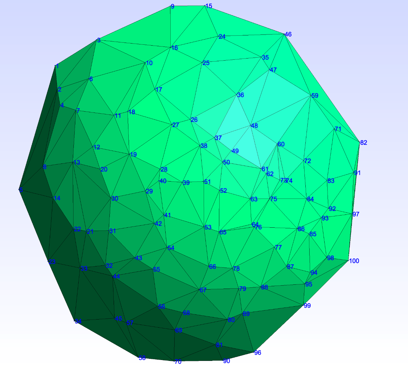
Fig. 26 Meshing produced from a thinned set of geostationary brightnessTemperature observations. See figure below for the spatial locations of the observations

The result of the application of the operator to a single observation (but with the mesh produced from the full set of observations shown in figure below) is shown below:

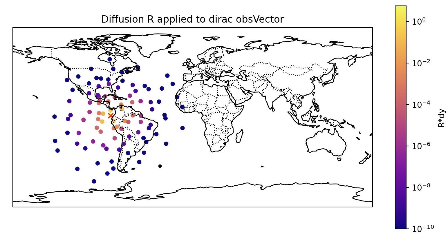
Fig. 27 The result of the diffusion operator being applied to a ‘dirac’ obsVector (a vector of all zero except for a single one) using the mesh from above.

Control Grid

In regions of sparse or irregular observations, Delaunay triangulation can produce unrealistically long-range connections between distant observation locations, leading to unphysical correlations in the diffusion operator.

An optional control grid can be added as scaffolding to guide the triangulation. A regular lon/lat grid is constructed at the specified resolution and any control grid points falling within a specified distance of an observation location are removed. The remaining control points are merged with the observation locations before mesh construction. Control grid points are assigned zero lengthscale so they guide the triangulation only and do not contribute to the diffusion.

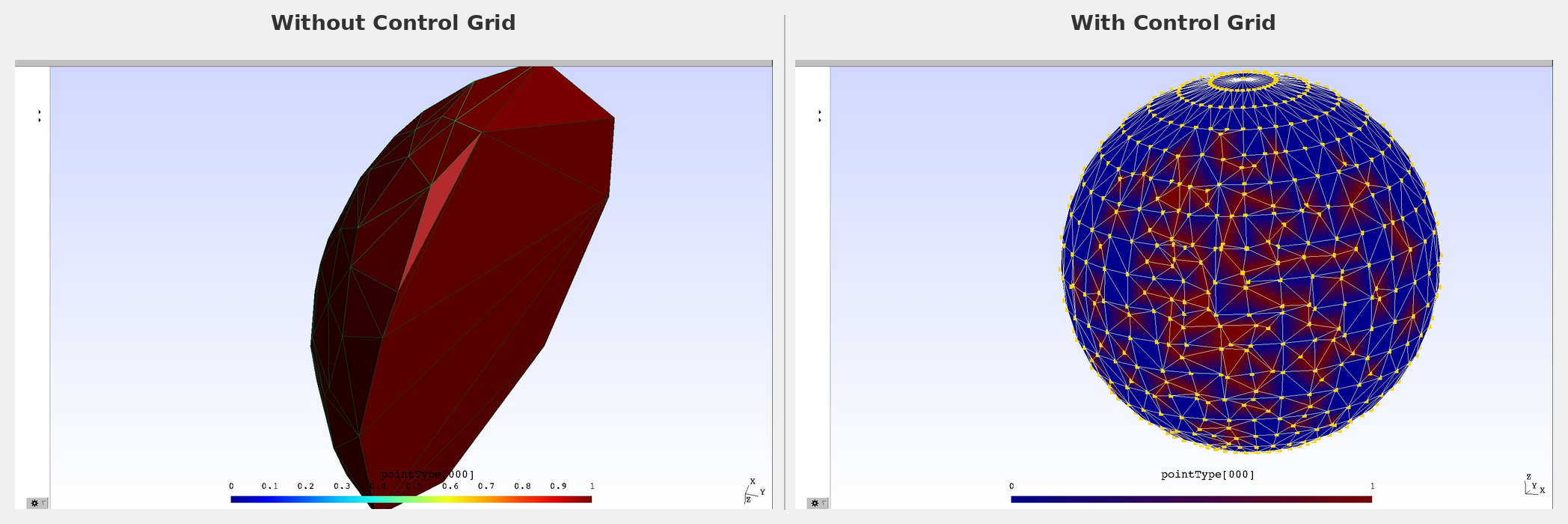
Fig. 28 Comparison of mesh without (left) and with (right) control grid for geostationary observations. Blue points indicate control grid points, red points indicate observation locations. The control grid eliminates the unrealistically long-range connections at the edges of the observation domain.

Note

For closely-spaced observations such as aircraft tracks, the control grid alone is not sufficient. Very small inter-observation distances cause the number of horizontal diffusion iterations to become very large. Gaussian thinning is recommended before applying this operator to such observation types.

The options for the operator include:

• correlation variable names: the names of variables to which the operator will be applied. Currently, this operator is only supported for use with a single variable.

• correlation lengthscale: length scale corresponding to the standard deviation of the gaussian profile this operator will emulate applying.

• normalization iterations: number of iterations used to calculate the set of grid-dependent normalization coefficients. See the documentation of the SABER Explicit Diffusion block for more details on the normalization procedure. For an operational/scientifically valid situation a value of at least ~10000 is recommended.

• control grid (optional): parameters for the optional control grid:

  • grid spacing: resolution of the control grid in degrees. Choose this carefully based on obs network geometry to avoid unwanted connections

  • remove within: distance threshold in meters. Control grid points within this distance of any observation location are removed.

Below is an example of a YAML configuration of the diffusion-based R operator with a control grid:

obs error:
  covariance model: diffusion
  correlation variable names: [brightnessTemperature]
  obs channels: [11]  #redundant with channels in obsSpace parameters
  correlation lengthscale: 200000. # meters
  normalization iterations: 10000
  control grid:
    grid spacing: 5      # degrees
    remove within: 50000 # meters