Rescaling Layer¶

General Description¶

The rescaling layer partially compensates for interpolation errors in a correlation or covariance model.

One of the most important characteristics of a covariance model is the variance field (the diagonal of the covariance matrix). When interpolating a covariance model from a source grid to a destination grid, the variance field is usually not preserved. Part of the signal is lost, which translates into a reduced variance. Typically, the user would want to preserve the variance during the interpolation, i.e. to have a covariance model on the destination grid whose variance field matches the field of the source variances interpolated to the destination grid. The rescaling layer applies a multiplicative correction, grid point by grid point, so that the variance field is effectively preserved during the interpolation.

This rescaling is very similar to the normalization step in BUMP-NICAS.

Relevance¶

This rescaling layer is only relevant:

in the context of covariance modeling.
when the correlation lengths are small or comparable to the source grid resolution.

This rescaling layer is not relevant:

In other contexts, for instance when interpolating ensemble perturbations.
When the correlation lengths are very large compared to the source grid resolution.

Example variance loss in idealized setting¶

Consider a homogeneous correlation model on a 1D grid with uniform spacing. After linear interpolation to a destination grid, the variance of the interpolated correlation model will be smaller than 1, with minimum values beign reached for destination points perfectly between two points of the source grid. In this case, the interpolated correlations decay to \((1+c)/2\), where \(c\) is the correlation at one-grid-cell distance.

This phenomenon is illustrated for a Gaussian correlation model in next figure.

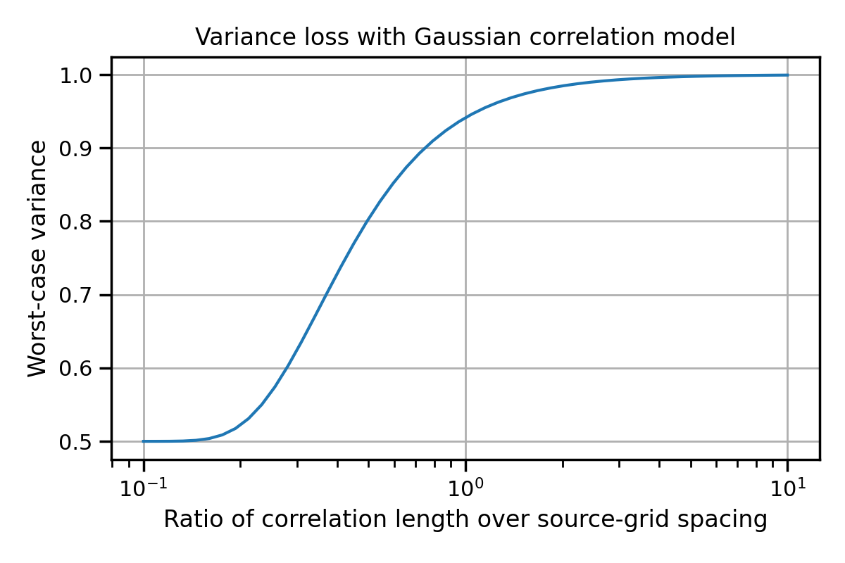
Variance loss in a 1D Gaussian correlation model

Fig. 4 Variance loss after interpolation of a 1D Gaussian correlation model¶

The maximum variance loss is 6% when the correlation length-scale is equal to the grid spacing, 20% when it is equal to half the grid spacing. In a 2D setting with bilinear interpolation, the variance is “lost” twice, so that the graph above can be read as a loss on standard-deviation rather than variances.

Mathematical Explanation¶

Suppose we want to interpolate a covariance model \(\mathbf{C}_S\) from a source grid \(S\) to a destination grid \(D\), using a linear operator \(\mathbf{T}\). The stencil of this linear operator can represent a linear interpolation, a bicubic interpolation etc.

\[\mathbf{C}_D = \mathbf{T} \mathbf{C}_S \mathbf{T}^T\]

Then the variance field of \(\mathbf{C}_D\) is given by its diagonal \(\mathbf{v}_D := \operatorname{Diag}(\mathbf{T} \mathbf{C}_S \mathbf{T}^T)\). This can be quite different from the original variances on the source grid \(\mathbf{v}_S := \operatorname{Diag}(\mathbf{C}_S)\). We cannot compare them directly, as they are defined on different grids. Interpolating the source variances to the destination grid gives the desired variance field: \(\mathbf{v}^*_D = \mathbf{T} \mathbf{v}_S\).

To correct the variance field, we compute a rescaling field \(\mathbf{r}\) such that the variances of the rescaled covariance model \(\mathbf{C}_D^* = \mathbf{R} \mathbf{C}_D\mathbf{R}^T\) (where \(\mathbf{R}\) is the diagonal matrix with diagonal \(\mathbf{r}\)) are the interpolated source variances.

This is achieved by defining

\[\forall i, \mathbf{r}_i = \sqrt{\frac{\mathbf{v}^*_{D i}}{\mathbf{v}_{D i}}} = \sqrt{\frac{(\mathbf{T} \mathbf{v}_S)_i}{(\mathbf{T} \mathbf{C}_S \mathbf{T}^T)_{ii}}}\]

Additive Rescaling¶

The multiplicative correction restores the variance of the covariance model, but it also affects the covariances. Another strategy could be to correct the variances only, by adding a diagonal matrix to the covariance model:

\[\mathbf{C}_D^* = \mathbf{C}_D + \mathbf{R}_+\mathbf{R}_+\]

where \(\mathbf{R}_+\) is a diagonal matrix with diagonal \(\mathbf{r}_+\), and where \(\mathbf{r}_+\) is defined as:

\[\forall i, \mathbf{r}_{+ i} = \sqrt{\mathbf{v}^*_{D i} - \mathbf{v}_{D i}}\]

Additive and multiplicative rescaling can also be combined to restore the full variance as:

\[\mathbf{C}_D^* = \mathbf{R} \mathbf{C}_D\mathbf{R}^T + \mathbf{R}_+\mathbf{R}_+\]

where

\[ \begin{align}\begin{aligned}\forall i, \mathbf{r}_i = \sqrt{\alpha\frac{\mathbf{v}^*_{D i}}{\mathbf{v}_{D i}} + (1-\alpha)}\\\forall i, \mathbf{r}_{+ i} = \sqrt{(1-\alpha)(\mathbf{v}^*_{D i} - \mathbf{v}_{D i})}\end{aligned}\end{align} \]

and where \(\alpha\) is the proportion of the variance that is restored multiplicatively.

Complexity of computing the rescaling field¶

The equations above are tractable if both numerator and denominator in the multiplicative rescaling coefficient can be computed in a linear time.

The numerator is the interpolated variance value, which is easy to derive provided the input variance field is known.

The denominator implies two matrix-matrix products. However, the sparsity of the interpolation operator \(\mathbf{T}\) can be exploited to reduce the three matrices involved in the computation to the size of the stencil of the interpolation operator:

\[\begin{split}(\mathbf{T} \mathbf{C}_S \mathbf{T}^T)_{ii} &= \mathbf{T}_{i, :} \mathbf{C}_S \mathbf{T}_{i, :}^T\\ &= \mathbf{T}_{i, J(i)} \mathbf{C}_{S [J(i), J(i)]} \mathbf{T}_{i, J(i)}^T\end{split}\]

where \(J(i)\) denotes the indexes of points in the stencil of the interpolation operator centered on grid point \(i\), i.e. the non-zero points in \(\mathbf{T}_{i, :}\).

We note that this assumes knowledge of the sub-matrices \(\mathbf{C}_{S [J(i), J(i)]}\) of short-scale covariances between all grid-points involved in a common stencil in the source grid, which may not be tractable in all cases.

User Guide for isotropic homogeneous covariance models¶

Step 1: Retrieve the short-scale covariances on the source grid

In the case of isotropic homogeneous covariance models, the short-scale covariances mentioned above can be retrieved from a 1D horizontal covariance profile for each model level.

Such vertical profiles can be retrieved using the covariance profile section in the Dirac test of The ErrorCovarianceToolbox Application. By defining a vertical column of Dirac point above a common horizontal location on the source grid and by disabling vertical convolutions in the covariance model, the 1D covariance profiles can be retrieved. For better accuracy, the Dirac test can be run in a zone where the grid is denser, or on a finer grid.

Here is an example of horizontal covariance profiles for a pressure variable.

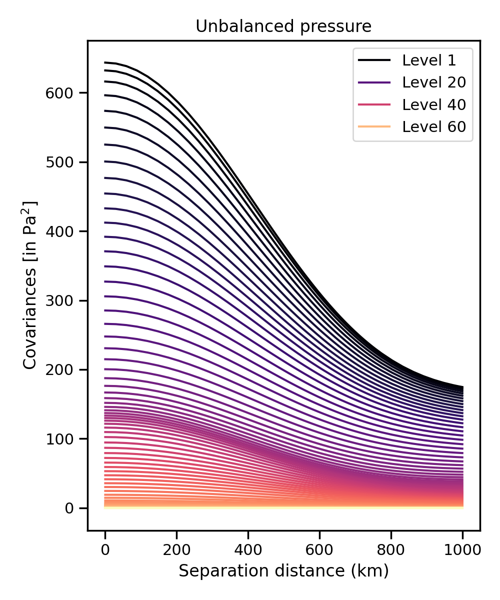
Fig. 5 Short-scale horizontal covariance profiles for unbalanced pressure.¶

Step 2: Compute and apply the rescaling field

The rescaling field can be computed from the short-scale covariances as described in the example yaml below.

- saber block name: gauss to cubed-sphere-dual
  gauss grid uid: F160
  rescaling:
    horizontal covariance profile file path: path/to/horizontal/covariance/profiles.nc
    active variables: <variables to rescale>
    fraction of lost variance to restore multiplicatively: 0.5  # Optional, defaults to alpha=1.0
    multiplicative coefficient atlas file:                      # Optional, needs alpha > 0
      filepath: path/to/output/multiplicative/rescaling/field
    additive coefficient atlas file:                            # Optional, needs alpha < 1
      filepath: path/to/output/additive/rescaling/field  # Can be reused as input of StdDev block

This will effectively compute the multiplicative and additive rescaling fields, and apply the multiplicative one.

Here is an example multiplicative rescaling field for a bilinear interpolation from a Gaussian grid with 20 points from Equator to pole to a cubed-sphere dual grid with 96 points per face. The signature of the source grid is clearly visible, with a smaller rescaling needed close to the source grid points. The latitudinal dependence reflects the higher density of source grid points near the Poles.

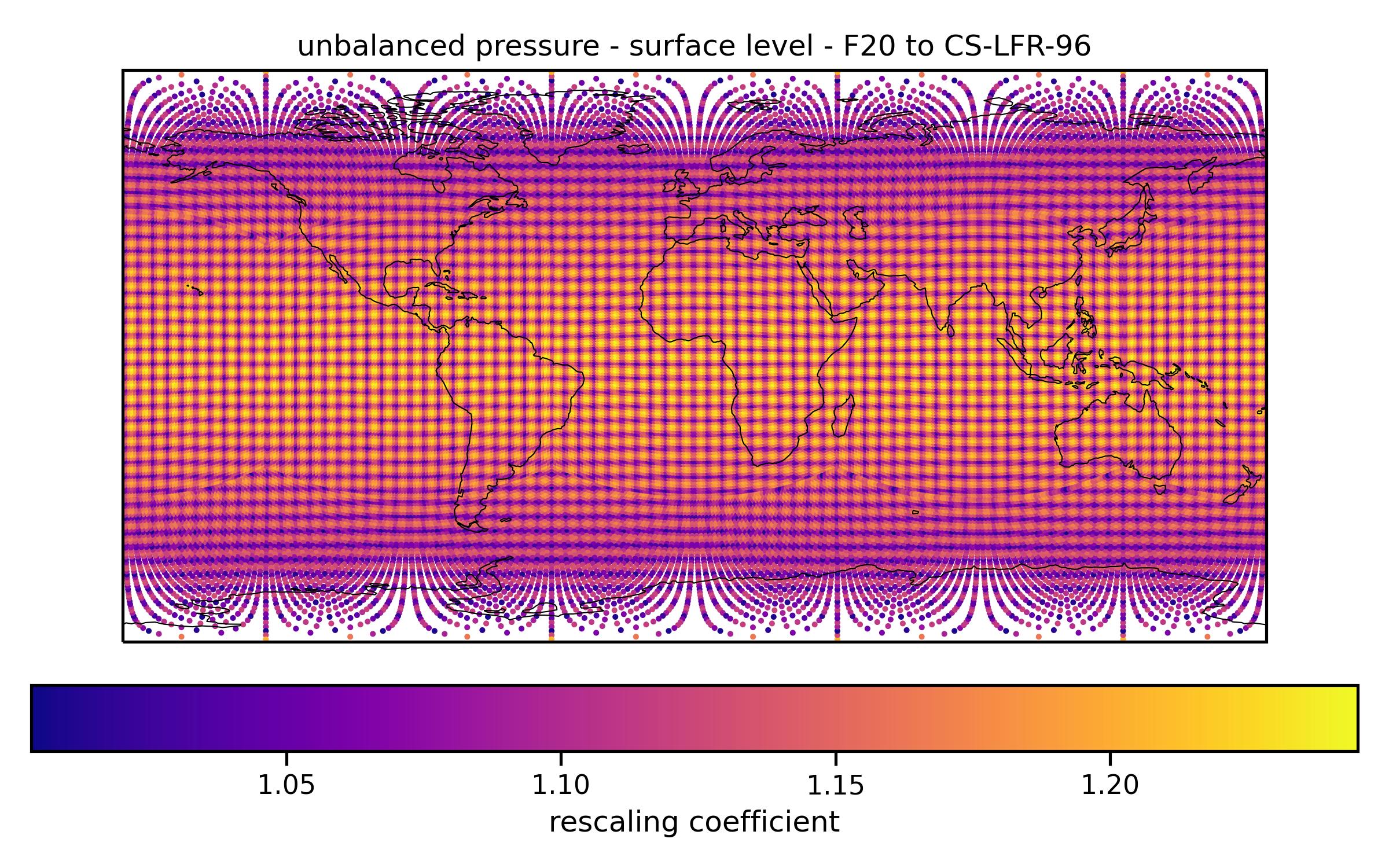
Rescaling field for a bilinear interpolation from a Gaussian grid to a cubed-sphere dual grid

Fig. 6 Rescaling field for a bilinear interpolation from a low-resolution Gaussian grid to a high-resolution cubed-sphere dual grid¶

Step 3: Read and apply the rescaling field

For further applications of the rescaling fields, the rescaling field output by a previous run can be read and applied directly using the following yaml.

- saber block name: gauss to cubed-sphere-dual
  gauss grid uid: F160
  rescaling:
    input atlas file:
      filepath: path/to/rescaling/field
    active variables: <variables to rescale>

Whether recomputing the field or reading it back from file is more efficient depends on the context.

Possible Improvements¶

Extension to the generic interpolation block: The rescaling layer is currently tied to the Gauss to cubed-sphere-dual interpolation. It should be extended to the generic “interpolation” saber block.
Extension to wind fields: The rescaling layer does not properly handles vector fields. The technique could possibly be extended to vector fields.
Using model I/O: The rescaling field could be output and read using the model I/O for higher efficiency.
More efficient look-up function: The look-up function to associate a separation distance to a covariance value could be made faster by returning covariance values for a full vertical column rather than being called for each horizontal level.
The short-scale covariances could also be informed by an analytical covariance profile (e.g., Gaussian with given length-scale) instead of read from file.