Write Variances
This block has two modes of use:
instantaneous statisticsmode - where horizontal global averaged variances are calculated for each model level. The data is from a single FieldSet at a specific point in the workflow. In all cases, when activated, it calculates binned variances from the FieldSet passed into theWriteVarianceblock’s class method(s) (multiply(),multiplyAD(), orleftInverseMultiply()) selected in the yaml configuration. This is to be used primarily for diagnostic purposes, and there is an option to write the variances to NetCDF files. In the near future, we will make this code more consistent with the other main mode.calibrationmode - where we accumulate using the “direct calibration” method. This method is still a work-in-progress and will be extended in the near future. Currently, it has the capability to generate variances, covariances, vertical-covariances, and vertical cross-covariances between 2 variables eitherat grid-points
as a globally horizontal-averaged quantity
or on over overlapping latitude bands.
In all cases we are assuming:
the mean of each field has been removed before entering this saber block. This affects the operations being performed.
the fields are either on a cubed-sphere dual mesh or on a classic Gaussian latitude mesh. The main restriction here is the need for a measure of the horizontal area for each grid point. In principle, we should be able to extend the usefulness of this block when we are able to get the horizontal area associated with each grid point from the model’s geometry.
in calibration mode we are assuming (for now) that the perturbations that are being used come from the randomization method. A consequence of this is that with this method there are N degrees of freedom with N perturbations, unlike the standard calculation where there are N-1 degrees of freedom for N perturbations (where one of the degrees of freedom has been used in calculating the ensemble mean as part of the process of creating the perturbations.)
Example yamls
There is an intentional limitation built into this saber block. Each instantiation of the block for the calibration will deal with only one type of statistics. Variances and covariance between two variables are both considered to have the statistics type = variances. Similarly vertical covariances and vertical cross-covariances are also grouped together with their statistics type = vertical covariances. Also, only one type of binning strategy (that is either “horizontal global average” or “horizontal grid point”) is allowed for each instantiation of the block.
Calculation of instantaneous statistics example is below. Note that at the moment the binning: key is required, even though instantaneous statistics mode is currently hard-coded to do horizontal global average binning (it computes the variance globally for each vertical level).
Note that the default statistics that are generated are variances and not vertical covariances
An example of instantaneous statistics.
saber outer blocks:
- (...)
- saber block name: write variances
  binning:                                                    // (required) binning category
    type: "horizontal global average"                         // (required) binning category type (NOT used with instantaneous statistics yet)
  field names: *vars                                          // list of variable names used calculating the variances or vertical covariances.
  instantaneous statistics:                                   // (optional) setting instantaneous statistics option
     multiply fset filename: <mult_file_name>                 // (optional) creating statistics every time going through multiply method.
     multiplyad fset filename: <multAD_file_name>             // (optional) creating statistics every time going through the adjoint of the multiply method.
     left inverse fset filename: <l_inv_file_name>            // (optional) creating statistics every time going through left inverse multiply method.
     output path: <path/to/output>                            // (required) path to where output files are written
- (...)
An example of vertical covariance calibration
saber outer blocks:
- (...)
- saber block name: write variances
  binning:                                                    // (required) binning category
    type: "horizontal global average"                         // (required) binning category type (NOT used with instantaneous statistics yet)
  calibration:                                                // (optional) switching on calibration
    write:                                                    // (optional) allow writing
      covariance name: "randomization with F12 mesh"          // (required) covariance name (used as a global header attribute) in the NetCDF file.
      mpi pattern: '%MPI%'                                    // mpi pattern string (needs %'s)
      file path: path2/vertcov_2_%MPI%.nc                     // file path for netCDF (total number of mpi ranks replace the %MPI%)
  field names: *vars                                          // list of variable names used calculating the variances or vertical covariances. (defaults to an empty vector of strings)
  statistics type: "vertical covariances"                     // statistics type (either "variances" (default) or "vertical covariances")
- (...)
An example of covariances between two variables on each grid point with binning information dumped to file
saber outer blocks:
- (...)
- saber block name: write variances
  additional cross covariances:                               // switching on cross covariances
  - variable 1: eastward_wind                                 // setting cross (co)variance between "eastward_wind" and "northward_wind"
    variable 2: northward_wind                                // both variable1 and variable2 are required.
  - variable 1: eastward_wind                                 // setting cross (co)variance between "eastward_wind" and "mu"
    variable 2: mu
  - variable 1: northward_wind                                // setting cross (co)variance between "northward_wind" and "mu"
    variable 2: mu
  binning:                                                    // (required) binning category
    type: "horizontal grid point"                             // (required) binning category type
    mpi rank pattern: '%MPI%'                                 // (optional) pattern but needed with filepath
    file path: path3/binning_data_%MPI%.nc                    // replaces %MPI% with MPI rank. One file is created for each MPI rank.
  calibration:                                                // (optional) switching on calibration
    write:                                                    // (optional) allow writing
      covariance name: "randomization with F12 mesh"          // (required) covariance name (used as a global header attribute) in the NetCDF file.
      mpi pattern: '%MPI%'                                    // mpi pattern string (needs %'s)
      file path: path2/intervariable_variances_%MPI%.nc       // file path for netCDF (total number of mpi ranks replace the %MPI%)
- (...)
An example of vertical covariances generated for overlapping latitude bands is below. This works for global domains only. The weights are calculated by multiplying the surface area associated with each grid point by a structure function that is dependent on latitude only and then is normalised so that the total sum of the weights across a bin sum to 1. There are a number of nodes (latitude points) that determine the extent and shape of the overlapping bands. The maximum and minimum latitude extent of each bin is given by \(-90 + (bin index + 1) * 180/(nbins)\) and \(-90 + (bin index ) * 180/(nbins)\) when \(bin index = 0, \cdots, nbins -1\) and \(nbins\) is the total number of bins. The maximum value of each structure function resides at the latitude that is the midpoint of the minimum and maximum latitudes for that bin. For bands that include either the North Pole or the South pole the structure function between the midpoint and the pole is constant. In all other cases, the structure function linearly decreases from the midpoint value to the values at the maximum and minimum extent.
saber outer blocks:
- (...)
- saber block name: write variances
  additional cross covariances:                               // switching on cross covariances
  - variable 1: eastward_wind                                 // setting cross (co)variance between "eastward_wind" and "northward_wind"
    variable 2: northward_wind                                // both variable1 and variable2 are required.
  - variable 1: eastward_wind                                 // setting cross (co)variance between "eastward_wind" and "mu"
    variable 2: mu
  - variable 1: northward_wind                                // setting cross (co)variance between "northward_wind" and "mu"
    variable 2: mu
  binning:
    type: "overlapping area-weighted latitude bands"
    no of bins: 7
    mpi rank pattern: '%MPI%'
    file path: path2/lat_overlap_binning_%MPI%.nc
  calibration:
    write:
      covariance name: "randomization with F12 mesh"
      mpi pattern: '%MPI%'
      file path: path/lat_overlap_vertcov_%MPI%.nc
  field names: *inputvars
  save NetCDF file: true
  statistics type:  "vertical covariance"
- (...)
Note that for the bins including the North or South poles the weighting function still drops as one approaches the pole, due to the decrease in the surface area associated with such points. Below are the weights accumulated on each of the Gaussian latitude rings. The plot below shows the accumulated weights for each latitude ring. For an F12 grid (with 24 Gaussian latitudes) and 7 bins, the sum of the weights on each Gaussian latitude is:
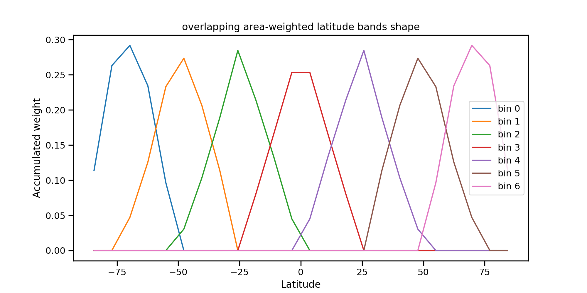
Fig. 4 Weights associated with each overlapping band.
General equations used
We are moving towards a generic binning strategy for variance/cross-covariance/vertical covariance/vertical cross-covariances. The description below will be limited to the case of a single processor element (PE). The considerations for the “domain decomposed” multiple PE case are described in the Technical implementation considerations section.
Let:
\(e\): the ensemble member index (and \(E\) is the ensemble size);
\(i\): the horizontal index associated with each field. In the context of covariances between 2 variables and vertical cross-covariances between 2 variables, we assume that this indexing is valid for the fields of both variables;
\(k\) be the model level index of each field;
\(\mathrm{fld1}(i,k)_e\): the first field for ensemble perturbation \(e\);
\(\mathrm{fld2}(i,k)_e\): the second field. When calculating variances and vertical covariances (and not covariances or vertical cross-covariances) both fields end up being the same;
\(b\): the bin index;
\(j\): index (starting at zero) of the horizontal points in each bin (with \(J\) bins in total). When calculating grid-point variances, we will have a bin of each grid point and \(J=1\);
\(\mathrm{binIdx}(b, j)\): the horizontal points used in each bin. So in the case of grid-point variances, the value of \(\mathrm{binIndx}(b, 0)\): the horizontal index associated with the bin \(b\);
\(\mathrm{w}(b, j)\): the normalized horizontal area for each grid point within each bin. We enforce that the total summed normalized horizontal area for each bin is equal to 1. When binning over the global domain the area associated with each grid point is normalized to be its fraction of the total area of the domain;
\(\mathrm{covar}(b,k)\): the (co)variance between two fields. When both fields are the same the equation reduces to calculating the variance;
\(\mathrm{vertcrosscov}(b,k_1,k_2)\): the vertical cross-covariance between two fields. Here we need a model level index for \(\mathrm{fld1}\) \(k_1\) and an associated level index for \(\mathrm{fld1}\) \(k_2\). When both fields are the same, the equation reduces to calculating the vertical covariance.
The limits of each index are denoted by capitalization.
The covariance is a generalisation of the variance calculation. To create the variance, field 1 and field 2 need to be the same.
Note that this only makes sense when both fields have the same number of model levels. (We do have an error trap to protect the user in that case).
The vertical cross-covariance is a generalisation of the covariance calculation (where \(\mathrm{covar}(b, k) = \mathrm{vertcrosscov}(b, k, k)\)).
NetCDF file specifications
The calibration covariance file is generated with a global NetCDF header of the form:
covariance name = "randomization with F12 mesh" ;
date time = "2010-01-01T12:00:00Z" ;
no of samples = 10 ;
The number of samples comes from the ensemble perturbations that have been read in. “date time” and “covariance name” come from the yaml.
The short name of each variable is the statistics type (“variance” or “vertical covariance”) followed by a variable index number.
Each NetCDF variable has its own set of variable attributes. An example of this for one variable is shown below. The variable attribute shows the covariance between variables “northward_wind” and “mu” in terms of horizontal global averages.
double variance 6(horizontal global average index, levels index 1) ;
  variance 6:_FillValue = -3.33476705790481e+38 ;
  variance 6:long_name = "variance of northward_wind and mu" ;
  variance 6:statistics type = "variance" ;
  variance 6:binning type = "horizontal global average" ;
  variance 6:variable name 1 = "northward_wind" ;
  variance 6:variable name 2 = "mu" ;
  variance 6:levels 1 = 70 ;
  variance 6:levels 2 = 70 ;
Another example is below:
double vertical covariance 5(horizontal global average index, levels index 1, levels index 2) ;
  vertical covariance 5:_FillValue = -3.33476705790481e+38 ;
  vertical covariance 5:long_name = "vertical covariance of eastward_wind and mu" ;
  vertical covariance 5:statistics type = "vertical covariance" ;
  vertical covariance 5:binning type = "horizontal global average" ;
  vertical covariance 5:variable name 1 = "eastward_wind" ;
  vertical covariance 5:variable name 2 = "mu" ;
  vertical covariance 5:levels 1 = 70 ;
  vertical covariance 5:levels 2 = 70 ;
We see that in this case the vertical cross-covariance between “eastward_wind” and “mu” is stored as a horizontal global average.
In addition we dump Binning data from each MPI rank to file. This is mainly for diagnostic uses. The global attributes of this file include the “binning type” and the “date time”. An example of the NetCDF header is below from the rank 1.
netcdf hor_gri_ave_1 {
dimensions:
  global PE bin index = 576 ;
  local PE bin index = 576 ;
  local PE horizontal point index = 1 ;
variables:
  double longitude(local PE bin index, local PE horizontal point index) ;
    longitude:_FillValue = -3.33476705790481e+38 ;
    longitude:long_name = "longitude" ;
    longitude:units = "degrees" ;
  double latitude(local PE bin index, local PE horizontal point index) ;
    latitude:_FillValue = -3.33476705790481e+38 ;
    latitude:long_name = "latitude" ;
    latitude:units = "degrees" ;
  double horizontal grid point weights(local PE bin index, local PE horizontal point index) ;
    horizontal grid point weights:_FillValue = -3.33476705790481e+38 ;
    horizontal grid point weights:long_name = "horizontal grid point weights" ;
    horizontal grid point weights:binning type = "horizontal grid point" ;
  int horizontal grid point global bins(global PE bin index) ;
    horizontal grid point global bins:_FillValue = -2147483643 ;

  // global attributes:
    :date time = "2010-01-01T12:00:00Z" ;
    :binning type = "horizontal grid point" ;
}
Here we store some of the information that we use within the BinningData_ fieldset (a member of the WriteVariance saber block class). The longitude and latitude values and the weights are given for each local bin index on the PE rank in question. Also a 1-dimensional array, called <binning_type> global bins, gives the global bin value for each local bin index on this PE rank and a 1-dimensional array, called <binning_type> horizontal extent, gives the number of horizontal points for each (local) bin on each PE rank. The variable horizontal grid point weights relates to the \(\mathrm{w}(b, j)\) in the equations above. We do not put the equivalent of \(\mathrm{binIdx}(b, j)\) into the NetCDF file. Instead we put the longitude and latitudes values associated to each horizontal index and each local bin index. In summary, we write \(\mathrm{longitude}(b, j)\), \(\mathrm{latitude}(b, j)\), \(\mathrm{w}(b, j)\), <binning_type> global bins and <binning_type> horizontal extent to a NetCDF file for each PE rank.
Technical implementation considerations
The main process in the calibration is to calculate the variances/vertical variances locally on each MPI rank for the bins that exist there and then to gather and sum this information onto processor rank 0. The data from a local MPI rank with a local bin index is mapped to the correct global index number as part of this process.