Toy Models in OOPS
Specific documentation
OOPS provides the following toy models that can be used in idealized experiments:
Unified plotting tool
Usage
The python script plot.py in oops/tools can be used to plot various diagnostics for the Lorenz95 and quasi-geostrophic models, with the following syntax:
python3 plot.py $MODEL $DIAG $GENERIC_ARGS $SPECIFIC_ARGS
- where:
$MODEL indicates the toy-model,
$DIAG indicates the diagnostic,
$GENERIC_ARGS is a sequence of generic arguments,
$SPECIFIC_ARGS is a sequence of model- and diagnostic-specific arguments.
Generic arguments:
$GENERIC_ARGS |
DESCRIPTION |
|---|---|
|
Print help message |
|
Optional output file name without extension |
Specific arguments:
$MODEL |
$DIAG |
$SPECIFIC_ARGS |
DESCRIPTION |
|---|---|---|---|
|
|
|
Log file path [.test or .log.out] |
|
|
NetCDF file path [.nc] |
|
|
Base NetCDF file path for difference [.nc] |
||
|
Background file path (optional for plot) [.nc] |
||
|
Truth file path (optional for plot) [.nc] |
||
|
Observations file path (optional for plot) [.nc] |
||
|
|
NetCDF file path (with %id% template) [.nc] |
|
|
Legend key for data from ‘filepath’ file (optional) |
||
|
NetCDF file path (with %id% template) [.nc] (optional) |
||
|
Legend key for data from ‘-f2’ file (optional) |
||
|
NetCDF file path (with %id% template) [.nc] (optional) |
||
|
Legend key for data from ‘-f3’ file (optional) |
||
|
NetCDF file path (with %id% template) [.nc] (optional) |
||
|
Legend key for data from ‘-f4’ file (optional) |
||
|
Truth file path (with %id% template) [.nc] |
||
|
Time series pattern values (used to replace %id%) |
||
|
|
Analysis file path [.nc] |
|
|
Truth file path [.nc] |
||
|
Background file path (optional for plot) [.nc] |
||
|
Recenter plot around first and last variable (optional) |
||
|
User specified title (optional) |
||
|
|
Analysis file path [.nc] |
|
|
Background file path [.nc] |
||
|
Truth file path (optional for plot) [.nc] |
||
|
Recenter plot around first and last variable (optional) |
||
|
User specified title (optional) |
||
|
|
|
Log file path [.test or .log.out] |
|
|
NetCDF file path [.nc] |
|
|
Base NetCDF file path for difference [.nc] |
||
|
Specify an observation file to plot the obs positions |
||
|
Flag to plot the wind |
||
|
Pattern replacing %id% in filepath to create a gif |
||
|
|
NetCDF file path [.nc] |
Examples
L95 / cost
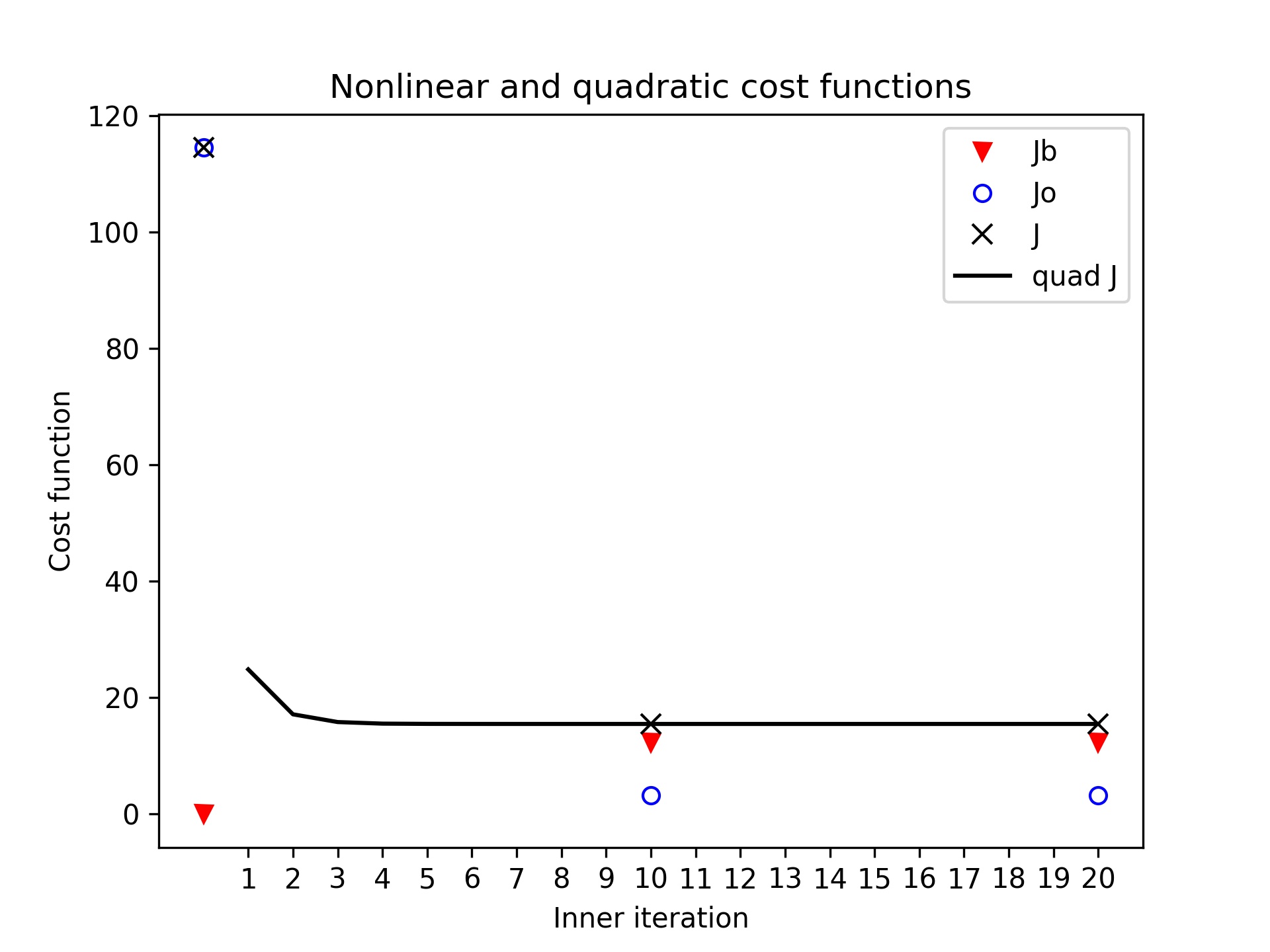
- Plot the cost function components for the 3DVar test of the L95 model:
red triangles: \(J_b\) term
blue circles: \(J_o\) term
black xs: \(J = J_b + J_o\)
black continuous line: \(quadratic J\) inside inner iterations
python plot.py l95 cost --output l95_cost \
               [build_bundle]/oops/l95/test/testoutput/3dvar.out
Parameters:
 - model: l95
 - diagnostic: cost
 - filepath: [build_bundle]/oops/l95/test/testoutput/3dvar.out
 - output: l95_cost
Run script
 -> plot produced: l95_cost.jpg
You will notice the quadratic function is flat, it is because the problem converges very fast.
L95 / fields
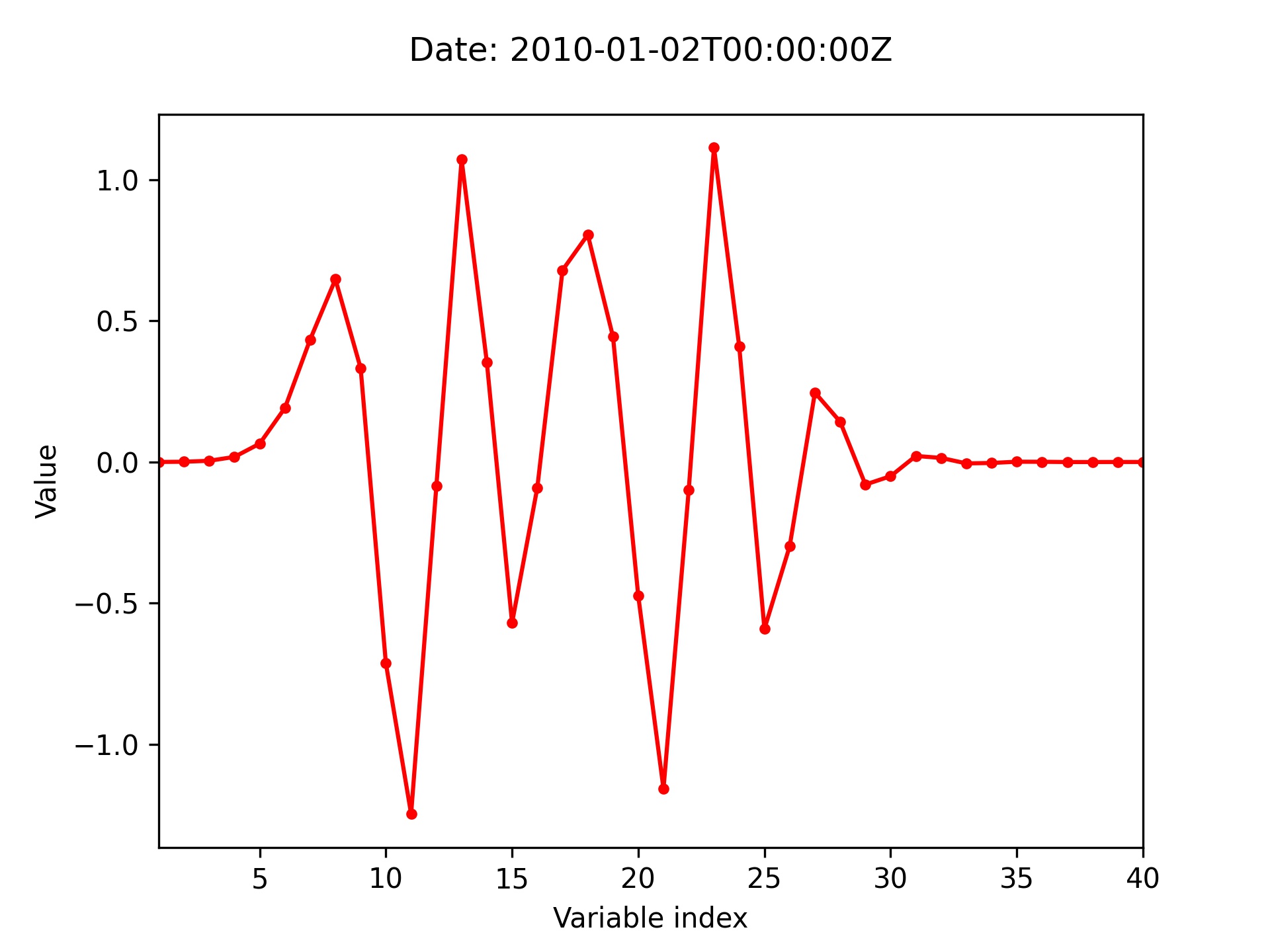
Plot the analysis increment (analysis - background) for the 3DVar test of the L95 model.
python plot.py l95 fields --output l95_fields \
               [build_bundle]/oops/l95/test/Data/3dvar.an.2010-01-02T00\:00\:00Z.l95 \
               [build_bundle]/oops/l95/test/Data/forecast.fc.2010-01-01T00\:00\:00Z.P1D.l95
Parameters:
 - model: l95
 - diagnostic: fields
 - filepath: [build_bundle]/oops/l95/test/Data/3dvar.an.2010-01-02T00:00:00Z.l95
 - basefilepath: [build_bundle]/oops/l95/test/Data/forecast.fc.2010-01-01T00:00:00Z.P1D.l95
 - output: l95_fields
Run script
 -> plot produced: l95_fields_incr.jpg
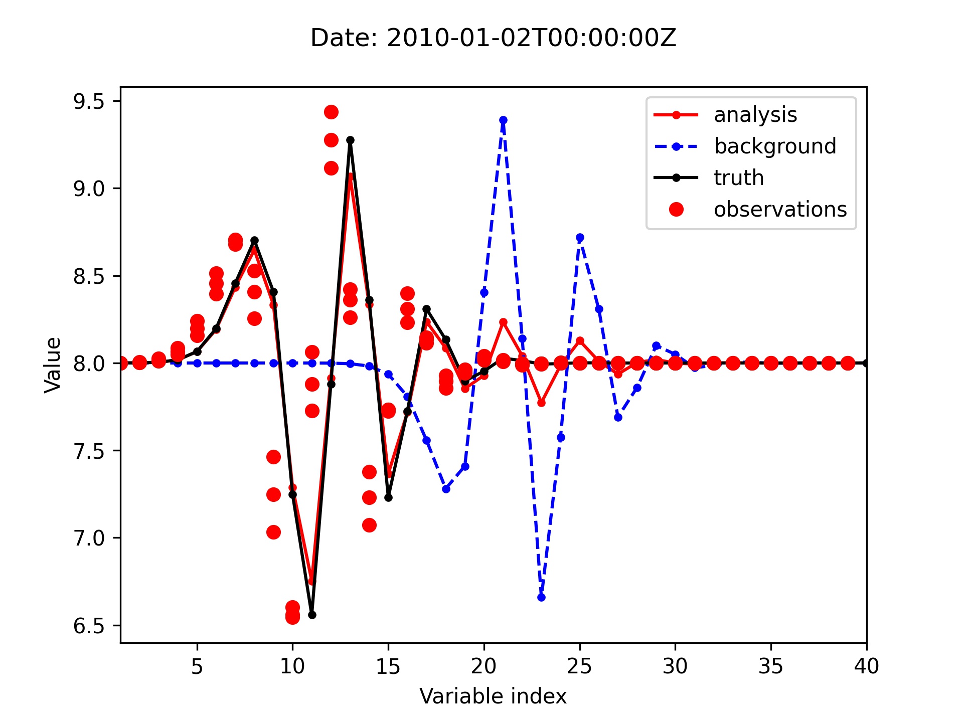
Plot the analysis, background, truth and observations for the 3DVar test of the L95 model.
python plot.py l95 fields [build_bundle]/oops/l95/test/Data/3dvar.an.2010-01-02T00\:00\:00Z.l95 \
               -bg [build_bundle]/oops/l95/test/Data/forecast.fc.2010-01-01T00\:00\:00Z.P1D.l95 \
               -t [build_bundle]/oops/l95/test/Data/truth.fc.2010-01-01T00\:00\:00Z.P1D.l95 \
               -o [build_bundle]/oops/l95/test/Data/truth3d.2010-01-02T00\:00\:00Z.obt

Parameters:
 - model: l95
 - diagnostic: fields
 - filepath: [build_bundle]/oops/l95/test/Data/3dvar.an.2010-01-02T00:00:00Z.l95
 - bgfilepath: [build_bundle]/oops/l95/test/Data/forecast.fc.2010-01-01T00:00:00Z.P1D.l95
 - truthfilepath: [build_bundle]/oops/l95/test/Data/truth.fc.2010-01-01T00:00:00Z.P1D.l95
 - obsfilepath: [build_bundle]/oops/l95/test/Data/truth3d.2010-01-02T00:00:00Z.obt
 - output: None
Run script
 -> plot produced: 3dvar.an.2010-01-02T00:00:00Z.jpg
Since several observations are available at each location throughout the time window, you can see up to three observation points for each location on the following plot.
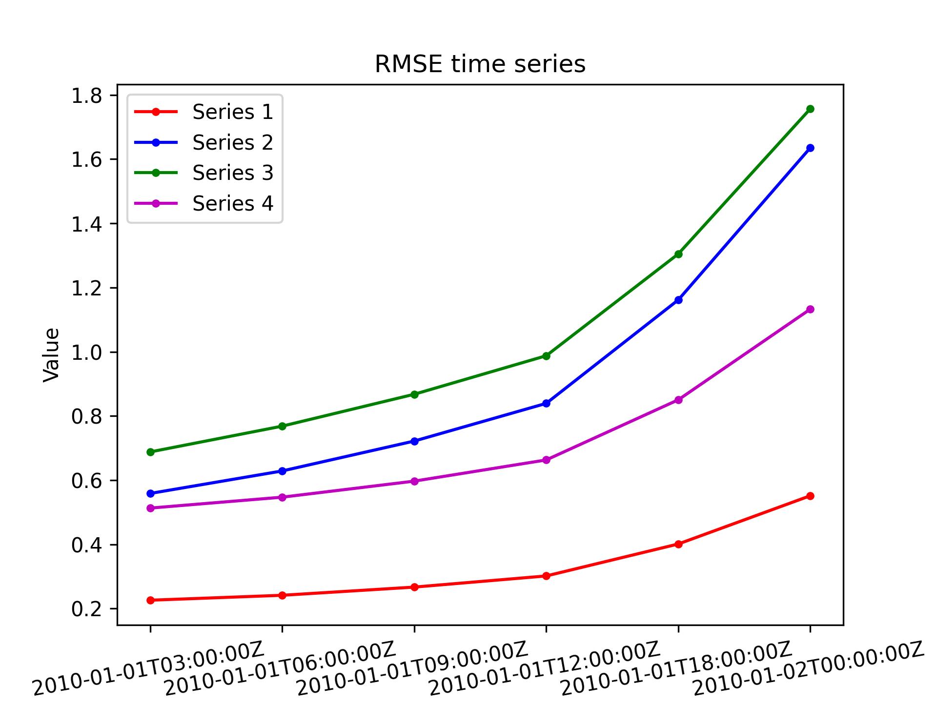
L95 / timeseries
Plot a time series of RMSE(field1 - field2) for DA tests using the L95 model. Optionally plot up to 3 more series with optional user specified legend keys.
python plot.py l95 timeseries [build_bundle]/oops/l95/test/Data/forecast.fc.2010-01-01T00\:00\:00Z.P%id%.l95 \
               -fKey "Series 1" \
               -f2 [build_bundle]/oops/l95/test/Data/forecast.ens.1.2010-01-01T00\:00\:00Z.P%id%.l95  \
               -f2Key "Series 2" \
               -f3 [build_bundle]/oops/l95/test/Data/forecast.ens.2.2010-01-01T00\:00\:00Z.P%id%.l95 \
               -f3Key "Series 3" \
               -f4 [build_bundle]/oops/l95/test/Data/forecast.ens.3.2010-01-01T00\:00\:00Z.P%id%.l95 \
               -f4Key "Series 4" \
               [build_bundle]/oops/l95/test/Data/truth.fc.2010-01-01T00\:00\:00Z.P%id%.l95 \
                T3H,T6H,T9H,T12H,T18H,1D

Parameters:
 - model: l95
 - diagnostic: timeseries
 - filepath: [build_bundle]/oops/l95/test/Data/forecast.fc.2010-01-01T00:00:00Z.P%id%.l95
 - fileKey: Series 1
 - filepath2: [build_bundle]/oops/l95/test/Data/forecast.ens.1.2010-01-01T00:00:00Z.P%id%.l95
 - file2Key: Series 2
 - filepath3: [build_bundle]/oops/l95/test/Data/forecast.ens.2.2010-01-01T00:00:00Z.P%id%.l95
 - file3Key: Series 3
 - filepath4: [build_bundle]/oops/l95/test/Data/forecast.ens.3.2010-01-01T00:00:00Z.P%id%.l95
 - file4Key: Series 4
 - truthfilepath: [build_bundle]/oops/l95/test/Data/truth.fc.2010-01-01T00:00:00Z.P%id%.l95
 - times: T3H,T6H,T9H,T12H,T18H,1D
 - output: None
Run script
 -> plot produced: forecast.fc.2010-01-01T00:00:00Z.P.jpg
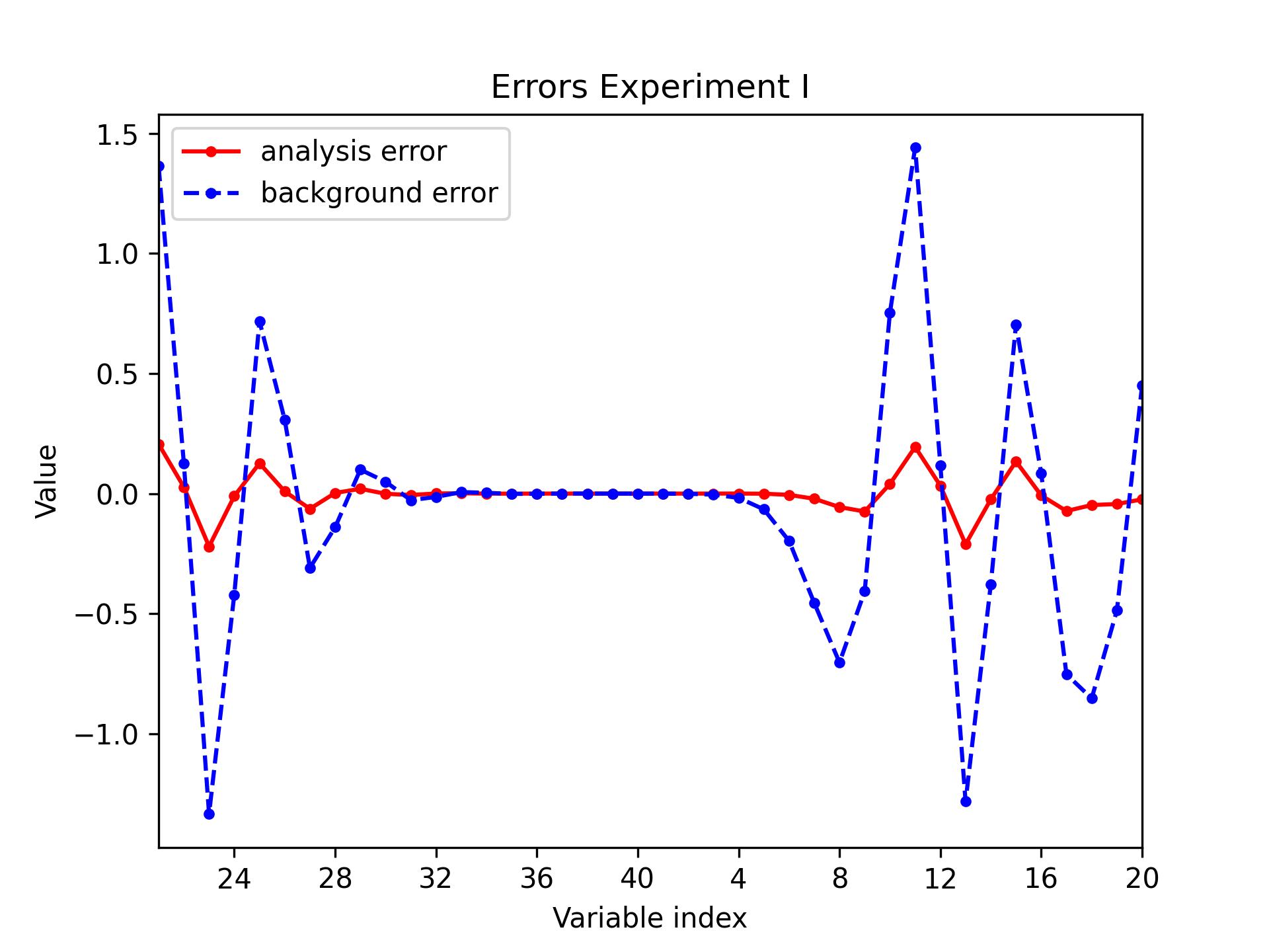
L95 / errors
Plot the following errors for the L95 model: analysis - truth (always) and background - truth (optionally).
python plot.py l95 errors [build_bundle]/oops/l95/test/Data/3dvar.an.2010-01-02T00\:00\:00Z.l95 \
               [build_bundle]/oops/l95/test/Data/truth.fc.2010-01-01T00\:00\:00Z.P1D.l95 \
               -bg [build_bundle]/oops/l95/test/Data/forecast.fc.2010-01-01T00\:00\:00Z.P1D.l95 \
               --recenter --title "Errors Experiment I"

Parameters:
 - model: l95
 - diagnostic: errors
 - filepath: [build_bundle]/oops/l95/test/Data/3dvar.an.2010-01-02T00\:00\:00Z.l95
 - truthfilepath: [build_bundle]/oops/l95/test/Data/truth.fc.2010-01-01T00\:00\:00Z.P1D.l95
 - bgfilepath: [build_bundle]/oops/l95/test/Data/forecast.fc.2010-01-01T00\:00\:00Z.P1D.l95
 - output: None
 - recenter: True
 - title Errors Experiment I
Run script
 -> plot produced: 3dvar.an.2010-01-02T00:00:00Z.jpg
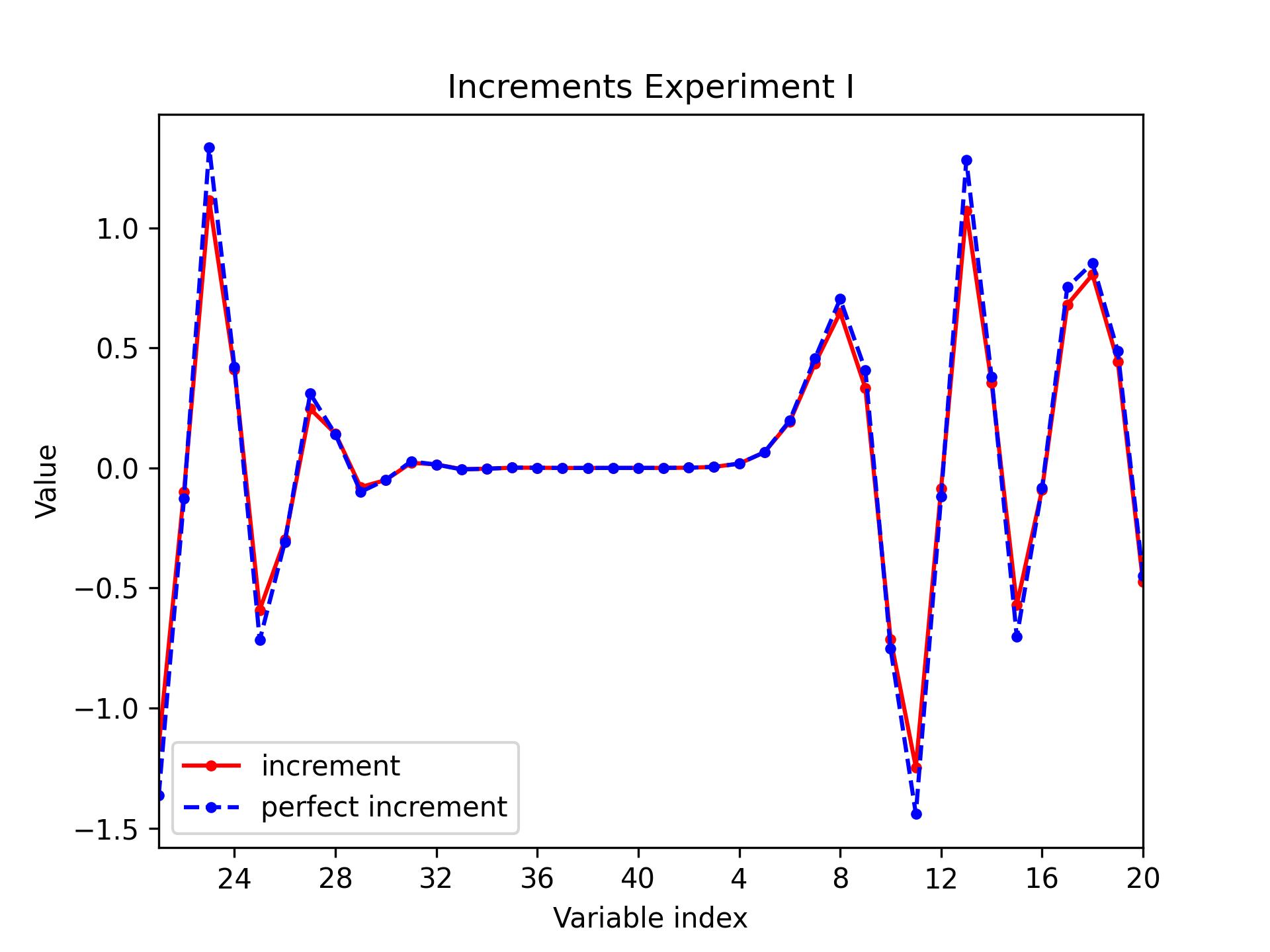
L95 / increments
Plot the following increments for the L95 model: increment analysis-background (always) and perfect increment truth - background (optionally).
python plot.py l95 increments [build_bundle]/oops/l95/test/Data/3dvar.an.2010-01-02T00\:00\:00Z.l95 \
               [build_bundle]/oops/l95/test/Data/forecast.fc.2010-01-01T00\:00\:00Z.P1D.l95 \
               -t [build_bundle]/oops/l95/test/Data/truth.fc.2010-01-01T00\:00\:00Z.P1D.l95 \
               --recenter --title "Increments Experiment I"

Parameters:
 - model: l95
 - diagnostic: increments
 - filepath: [build_bundle]/oops/l95/test/Data/3dvar.an.2010-01-02T00:00:00Z.l95
 - bgfilepath: [build_bundle]/oops/l95/test/Data/forecast.fc.2010-01-01T00:00:00Z.P1D.l95
 - truthfilepath: [build_bundle]/oops/l95/test/Data/truth.fc.2010-01-01T00:00:00Z.P1D.l95
 - output: None
 - recenter: True
 - title: Increments Experiment I
Run script
 -> plot produced: 3dvar.an.2010-01-02T00:00:00Z.jpg
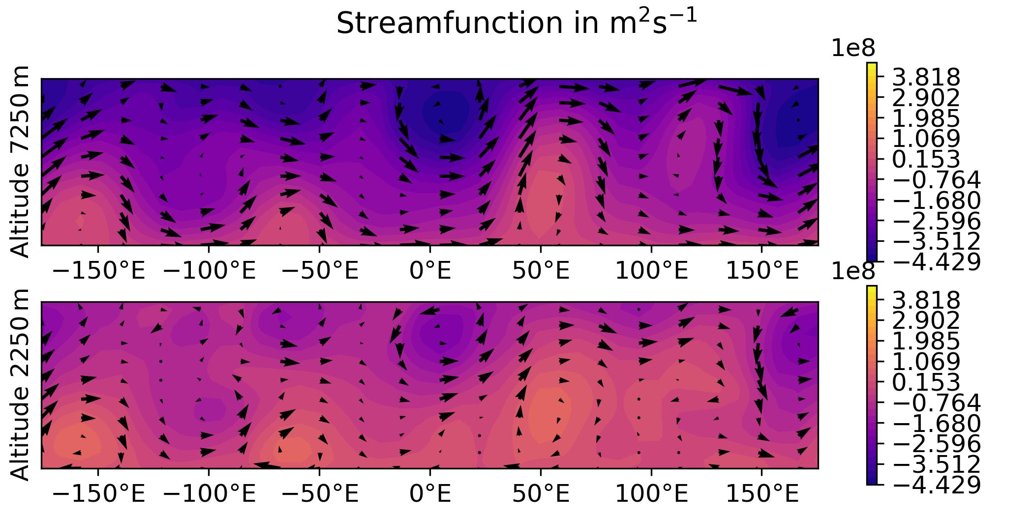
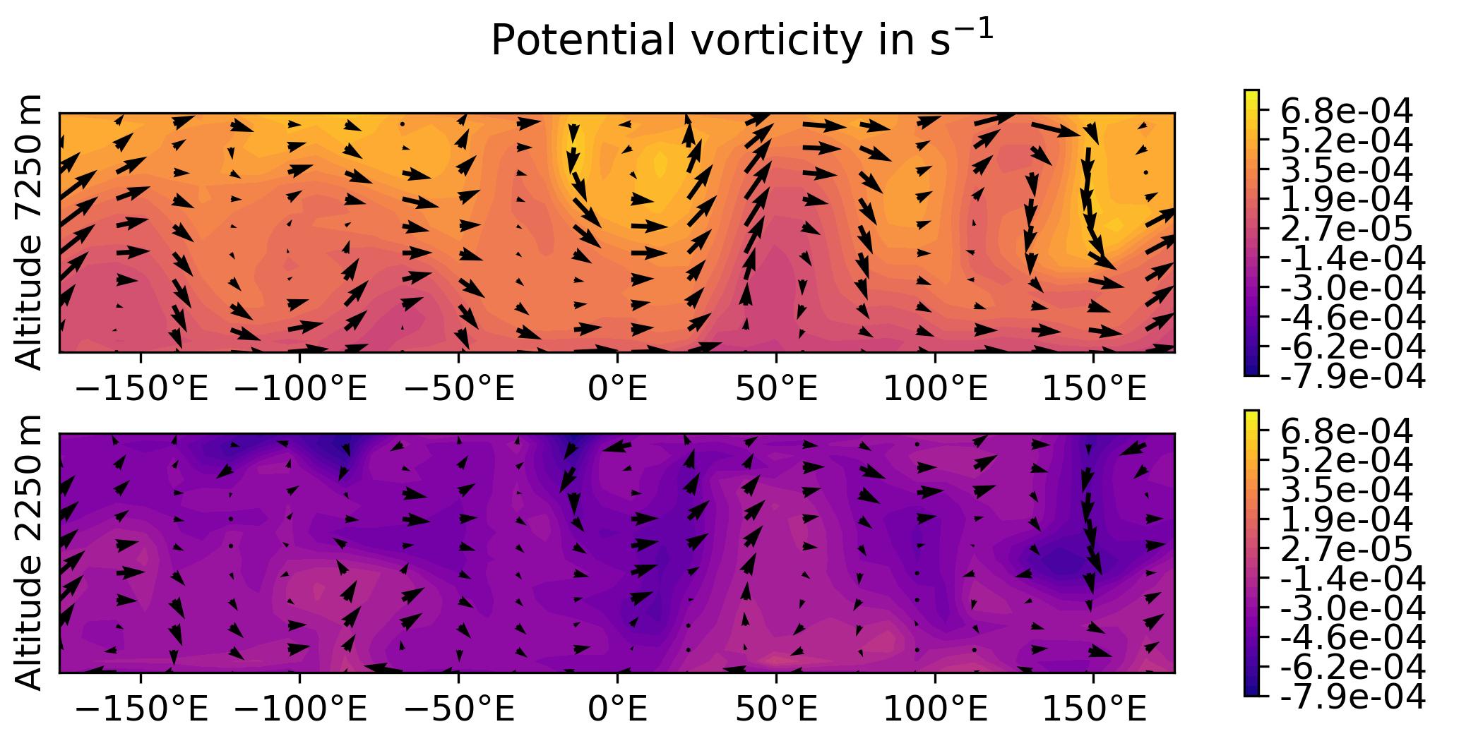
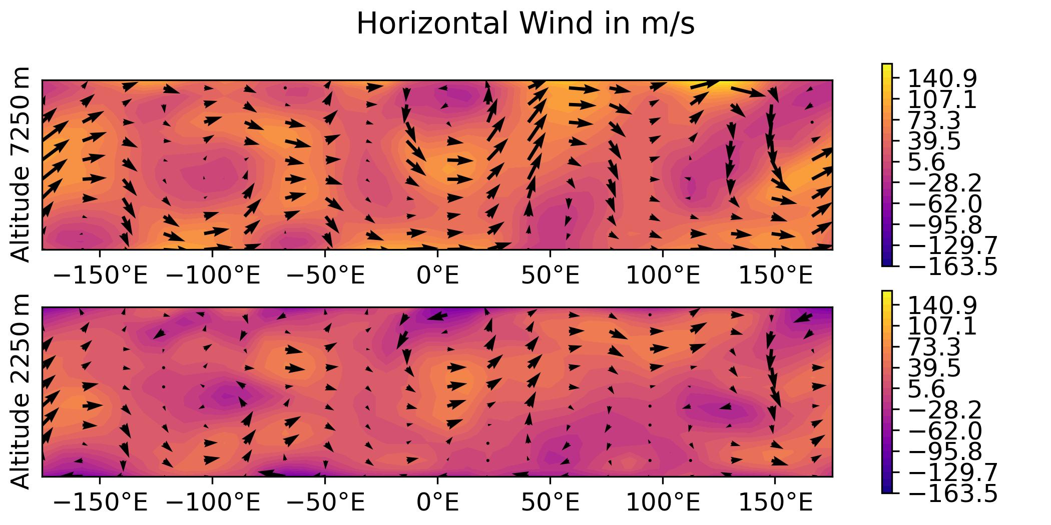
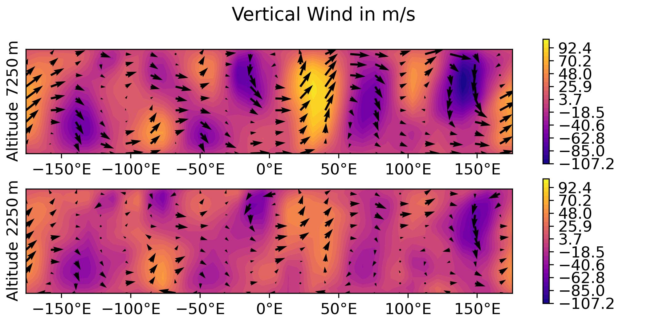
QG / fields
- Plot the analysis for the 3DVar test of the QG model, with corresponding geostrophic winds:
streamfunction on levels 1 and 2,
potential vorticity on levels 1 and 2.
horizontal wind on levels 1 and 2.
vertical wind on levels 1 and 2.
python plot.py qg fields --output qg_fields \
               [build_bundle]/oops/qg/test/Data/3dvar.an.2010-01-01T12\:00\:00Z.nc
Parameters:
 - model: qg
 - diagnostic: fields
 - filepath: [build_bundle]/oops/qg/test/Data/3dvar.an.2010-01-01T12:00:00Z.nc
 - basefilepath: None
 - plotObsLocations: None
 - plotwind: False
 - gif: None
 - output: qg_fields
 - title: None
Run script
 -> plot produced: qg_fields_x.jpg
 -> plot produced: qg_fields_q.jpg
 -> plot produced: qg_fields_u.jpg
 -> plot produced: qg_fields_v.jpg
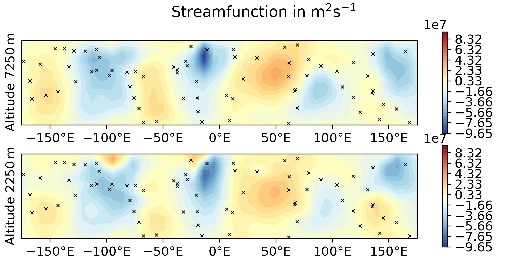
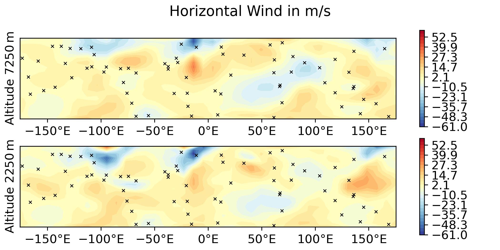
QG / fields - increment and overlay observation positions
Plot the increment for the 3DVar test of the QG model and overlay the observation locations:
python plot.py qg fields --output qg_increment \
               --plotwind \
               [build_bundle]/oops/qg/test/Data/3dvar.an.2010-01-01T12\:00\:00Z.nc \
               [build_bundle]/oops/qg/test/Data/forecast.fc.2009-12-31T00\:00\:00Z.P1DT12H.nc \
               --plotObsLocations [build_bundle]/oops/qg/test/Data/truth.obs3d.nc
Parameters:
 - model: qg
 - diagnostic: fields
 - filepath: [build_bundle]/oops/qg/test/Data/3dvar.an.2010-01-01T12:00:00Z.nc
 - basefilepath: [build_bundle]/oops/qg/test/Data/forecast.fc.2009-12-31T00:00:00Z.P1DT12H.nc
 - plotObsLocations: [build_bundle]/oops/qg/test/Data/truth.obs3d.nc
 - plotwind: True
 - gif: None
 - output: qg_increment
 - title: None
Run script
 -> plot produced: qg_increment_x_diff.jpg
 -> plot produced: qg_increment_q_diff.jpg
 -> plot produced: qg_increment_u_diff.jpg
 -> plot produced: qg_increment_v_diff.jpg
QG / fields - animated GIF
Plot the sequence of states of the “truth” forecast in an animated GIF.
python plot.py qg fields --output qg_fields_animation_%id% \
               [build_bundle]/oops/qg/test/Data/truth.fc.2009-12-15T00\:00\:00Z.%id%.nc \
               --gif P1D,P2D,P3D,P4D,P5D,P6D,P7D,P8D,P9D,P10D,P11D,P12D,P13D,P14D,P15D,P16D,P17D,P18D
Parameters:
 - model: qg
 - diagnostic: fields
 - filepath: [build_bundle]/oops/qg/test/Data/truth.fc.2009-12-15T00:00:00Z.%id%.nc
 - basefilepath: None
 - plotObsLocations: None
 - plotwind: False
 - gif: P1D,P2D,P3D,P4D,P5D,P6D,P7D,P8D,P9D,P10D,P11D,P12D,P13D,P14D,P15D,P16D,P17D,P18D
 - output: qg_fields_animation_%id%
 - title: None
Run script
 -> plot produced: qg_fields_animation_P1D_x.jpg
 -> plot produced: qg_fields_animation_P2D_x.jpg
 -> plot produced: qg_fields_animation_P3D_x.jpg
 -> plot produced: qg_fields_animation_P4D_x.jpg
 -> plot produced: qg_fields_animation_P5D_x.jpg
 -> plot produced: qg_fields_animation_P6D_x.jpg
 -> plot produced: qg_fields_animation_P7D_x.jpg
 -> plot produced: qg_fields_animation_P8D_x.jpg
 -> plot produced: qg_fields_animation_P9D_x.jpg
 -> plot produced: qg_fields_animation_P10D_x.jpg
 -> plot produced: qg_fields_animation_P11D_x.jpg
 -> plot produced: qg_fields_animation_P12D_x.jpg
 -> plot produced: qg_fields_animation_P13D_x.jpg
 -> plot produced: qg_fields_animation_P14D_x.jpg
 -> plot produced: qg_fields_animation_P15D_x.jpg
 -> plot produced: qg_fields_animation_P16D_x.jpg
 -> plot produced: qg_fields_animation_P17D_x.jpg
 -> plot produced: qg_fields_animation_P18D_x.jpg
 -> gif produced: qg_fields_animation_P1D_x.gif
 -> plot produced: qg_fields_animation_P1D_q.jpg
 -> plot produced: qg_fields_animation_P2D_q.jpg
 -> plot produced: qg_fields_animation_P3D_q.jpg
 -> plot produced: qg_fields_animation_P4D_q.jpg
 -> plot produced: qg_fields_animation_P5D_q.jpg
 -> plot produced: qg_fields_animation_P6D_q.jpg
 -> plot produced: qg_fields_animation_P7D_q.jpg
 -> plot produced: qg_fields_animation_P8D_q.jpg
 -> plot produced: qg_fields_animation_P9D_q.jpg
 -> plot produced: qg_fields_animation_P10D_q.jpg
 -> plot produced: qg_fields_animation_P11D_q.jpg
 -> plot produced: qg_fields_animation_P12D_q.jpg
 -> plot produced: qg_fields_animation_P13D_q.jpg
 -> plot produced: qg_fields_animation_P14D_q.jpg
 -> plot produced: qg_fields_animation_P15D_q.jpg
 -> plot produced: qg_fields_animation_P16D_q.jpg
 -> plot produced: qg_fields_animation_P17D_q.jpg
 -> plot produced: qg_fields_animation_P18D_q.jpg
 -> gif produced: qg_fields_animation_P1D_q.gif
QG / obs
Copy the observation file values from the NetCDF into a text file.
python plot.py qg obs --output qg_obs [build_bundle]/oops/qg/test/Data/3dvar.obs3d.nc
Parameters:
 - model: qg
 - diagnostic: obs
 - filepath: [build_bundle]/oops/qg/test/Data/3dvar.obs3d.nc
 - output: qg_obs
Run script
 -> Observations values written in qg_obs.txt
File extract:
# location / value / hofx
[ -29.87208056    3.63767342 3266.44902118] / [10594165.5105961] / [10594165.5105961]
[ 178.98653093    8.23197272 5786.33931931] / [-876673.14254443] / [-876673.14254443]
[  79.31681614   59.17619073 5270.58105916] / [-1.33785214e+08] / [-1.33785214e+08]
...
[  30.72931674   18.82485907 6153.04231877] / [56.26459124] / [56.26459124]