Diagnostics
The purpose of this package is to help developers and users evaluate MPAS-JEDI performance, and diagnose potential errors in the system. The package includes scripts for plotting the cost function, the norm of the gradient, observation distribution, and analysis increment. To support testing of EDA with MPAS-JEDI, the package includes probabilistic evaluations of the ensemble of background forecasts. It also includes observation- and model-space verification tools for tracking the performance of cycling experiments. Those tools evaluate traditional statistical measures (Mean, RMS, standard deviation, etc…) for surface and upper air variables. Additionally there is some capability for determining confidence intervals for those verification measures. Both the model- and observation-space components provide a means to store intermediate statistical measures and then visualize verification statistics.
Cartopy, matplotlib, numpy, h5py, and netCDF4 Python packages are required to perform the diagnostics.
Analysis Increments
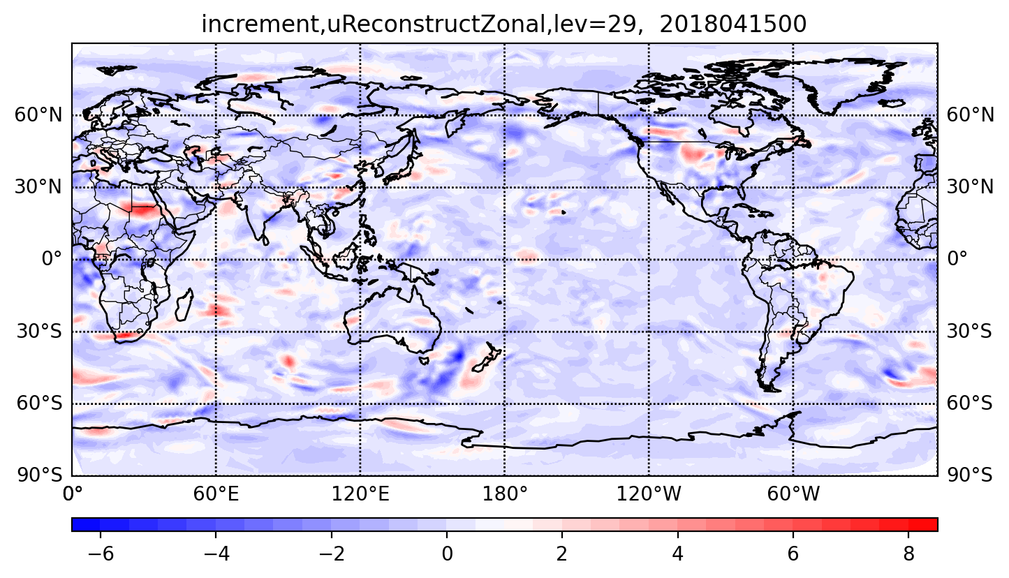
A plot of analysis increments can help users to understand how the model analysis has adjusted to
assimilated observations. You can calculate the analysis increment and make figures for different
analysis fields by using mpas-bundle/mpas-jedi/graphics/plot_inc.py. The following example is for
visualizing the analysis increment of the zonal component of reconstructed horizontal velocity.
python $GRAPHICS_DIR/plot_inc.py $DATE 3denvar uReconstructZonal 1 False
The argument 1 means the analysis increment will be plotted by each level, and
the argument False means the MPAS analysis will not be compared with corresponding GFS analysis.
The following figure shows zonal wind increment at 0000 UTC 15 Apr 2018 on the 29th model level.
Observation-space verification
All scripts discussed in this section are located in GRAPHICS_DIR/cycling, where
GRAPHICS_DIR = mpas-bundle/mpas-jedi/graphics.
MPAS-JEDI utilizes the IODA and UFO file writing mechanisms to generate observation-space feedback
files from hofx and variational applications. That includes the standard IODA ObsSpace as well as
optional GeoVaLs and ObsDiagnostics. The standard IODA ObsSpace is written using the ObsSpace::save method in IODA,
while GeoVaLs and ObsDiagnostics are written using the GeoVaLs::write method in UFO.
The sample yaml setting to output the feedback file for hofx is as follows:
obsdataout:
  engine:
    type: H5File
    obsfile: dbOut/obsout_hofx_sondes.h5
and for variational:
obsdataout:
  engine:
    type: H5File
    obsfile: dbOut/obsout_variational_sondes.h5
In the Variational application, ObsGroups associated with EffectiveQC, EffectiveError, hofx, and ObsBias are saved with iteration number, such as EffectiveQC0, EffectiveQC1, which is not the case for the HofX application.
Those database files feed into a robust observation-space
python-based verification tool. The first part of the tool diagnoses fits to observations, and
writes binned statistics to intermediate NetCDF database files. If you perform verification on NCAR
CISL’s Derecho HPC, run the ncar_pylib command first in order to load all of the required python
modules.
Below is a sample shell script for writing the intermediate statistics database file for a single time.
mkdir diagnostic_stats
cd diagnostic_stats
ln $GRAPHICS_DIR/cycling/*.py .
python DiagnoseObsStatistics.py -n $NumProcessors -p $ObsSpaceDirectory -app hofx -o obsout -g geovals -d ydiag >& diags.log
NumProcessors is the number of processors available, each of which processes a different
observation type. For large data sets, this may need to be smaller than the number of processors on
a node due to memory overhead. ObsSpaceDirectory is the location of the observation
feedback files. The app argument can either be hofx or variational,
depending on which generic application was used to generate the data. The user can select the
prefixes of the different types of database files with the -o, -g, and -d
arguments. Additional requirements for file naming conventions are described in JediDB.py.
For example, this code is currently designed to handle multi-processor output with a process rank
suffix, each process having written its own file corresponding to a subset of the locations.
DiagnoseObsStatistics.py generates one file per diagnosed observation type, each having the
stats_ prefix.
After statistics are created for more than one valid date, the analysis configuration script,
analyze_config.py, gives directions for generating figures from a set of statistics files
across multiple valid dates. Settings such as user, dbConf['expLongNames'], and
dbConf['DAMethods'] need to match the directory structure of your workflow system.
dbConf['expNames'] is used to assign shorter label names for each experiment.
dbConf['cntrlExpIndex'] is used to choose which experiment is considered the control in
difference plots. Variables such as the first and last cycle dates and increment as well as the
first and last forecast durations and increment should also be modified.
Users can then run AnalyzeStats.py on the command-line or submit many jobs, each one for a
different observation type, using SpawnAnalyzeStats.py. This procedure is described in
detail in analyze_config.py. Take note that the automated job submission process is only
enabled on CISL’s Derecho and Casper login nodes at this time.
Model-space verification
Model-space verification can be used to verify an analysis or a forecast against gridded fields (e.g., GFS analyses).
Input files are GFS analyses (or other source) in MPAS grid and MPAS analyses or forecasts. Users can use a shell script to control model-space verification,
and the modelsp_utils.py includes variables needed when you setup environment variables in the shell script,
such as expLongNames, initDate, endDate, intervalHours, fcHours, etc.
The sample shell script for write diagnostics and visualize verification statistics looks like:
mkdir diagnostic_stats
cd diagnostic_stats
# Write diagnostics in NetCDF format.
python $GRAPHICS_DIR/writediag_modelspace.py
# Plot 2-D figures for upper air variables.
python $GRAPHICS_DIR/plot_modelspace_ts_2d.py
# Plot 1-D figures for surface variables.
python $GRAPHICS_DIR/plot_modelspace_ts_1d.py
Here, diagnostic_stats is a subdirectory in your forecast directory. Users wishing to compute aggregated statistics across cycling period can use the following commands:
# Compute aggregated statistics and write diagnostics in NetCDF format.
python $GRAPHICS_DIR/writediag_modelspace_aggr.py
# Plot aggregated statistics for upper air variables.
python $GRAPHICS_DIR/plot_modelspace_aggr.py
# Plot aggregated statistics for surface variables.
python $GRAPHICS_DIR/plot_modelspace_ts_1d_aggr.py