Tutorial: Working with IODA through the Python API
- Learning Goals:
Gain insight into the IODA data model through the Python API
Learn how to read a IODA file into python for plotting and diagnostics
- Prerequisites:
read the tutorial overview
familiarity with python programming
Overview
The Interface for Observational Data Assimilation (IODA) is the component of JEDI that handles observational data. The principle software design objective that guides IODA development is what is known in the software engineering world as the separation of concerns. In short, developers who are implementing new DA algorithms or interfacing new models into JEDI should not need to worry about the details of how observational data is organized in files. Conversely, scientists and developers who are integrating new observational instruments into JEDI need not concern themselves with the details of how these observational data will be used. This separation of concerns is achieved through an abstract data model that is implemented through a generic set of interfaces; what programmers call an API (Application Programming Interface).
The IODA data model is based on the HDF5 Data Model both in its high-level design and its low-level implementation. HDF5 (Hierarchical Data Format, version 5) is a well-established standard in the high-performance computing (HPC) community for for efficient processing and storage of large data volumes. HDF5 also forms the basis of the popular NetCDF (version 4) file format that is widely used in the weather forecasting community.
That is not to say that IODA relies on HDF5 or NetCDF4 for its input. In the code component we call ioda-engines, we separate out how the data are stored (the backend engine) from how an end user can access it (the frontend engine). The same frontend API can thus access data through a variety of file formats and other data channels, implemented as backend engines. As IODA development proceeds, we expect the diversity of supported backend engines to continue to grow.
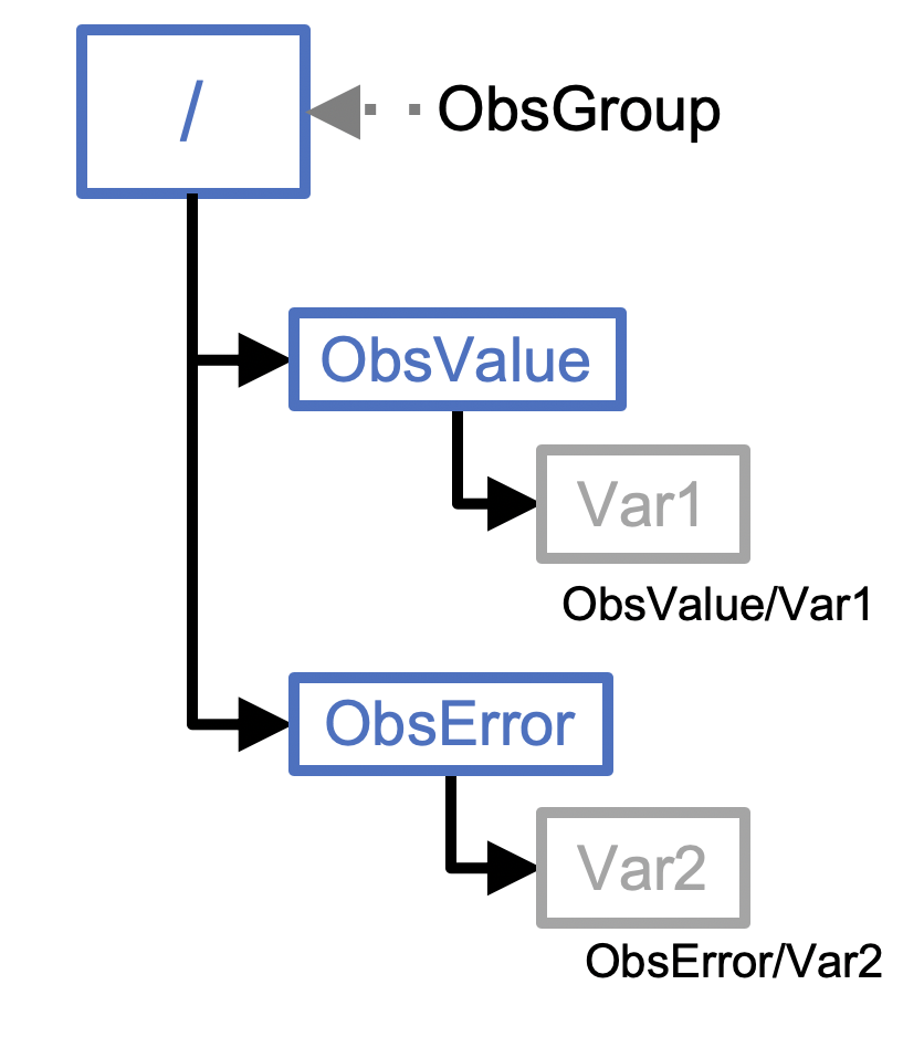
Data in IODA are stored in a structure Groups, Variables, and Attributes. A Group is like a folder. It is a logical collection of Variables and Attributes that describes some portion of the overall data. A Variable stores bulk data. An Attribute stores smaller quantities of metadata, and can be attached to either a Group or a Variable. Groups can be nested.
The following figure illustrates this organization. Observational data for a particular instrument and time interval is stored in one or more variables, here represented as Var1. The variables are organized into a group called ObsValue. Each measurement has an associated error estimate, which is similarly represented by one or more variables and organized into a group called ObsError. These are then combined into a top-level ObsGroup represented here by a /. Other groups may also be included in the ObsGroup, including ObsBias and PreQC. Attributes can then be added at the ObsGroup level, at the nested group level, or even at the variable level, as appropriate. Though Attributes can contain a diverse range of metadata, it is often beneficial to also include a separate MetaData group within the ObsGroup for additional metadata that may have distinct values for each of the data points. Examples include latitude, longitude, and date/time.
The IODA data model is implemented through abstract base classes in C++. This leverages the generic, object-oriented capabilities of the C++ language to allow for multiple implementations. An added benefit is these base classes can be accessed from python through a package called pybind11. They can also be accessed from Fortran through the ISO_C_BINDING.
In this tutorial we will explore the IODA data model through the python API.
Step 1: Enter the Container
If you have already done the Run JEDI in a Container tutorial then you already have downloaded and verified the JEDI tutorial container. Navigate to that directory and re-enter the container, if you are not already there:
singularity shell -e jedi-tutorial_latest.sif
If you have not done that tutorial then do it now to gain access to the tutorial container.
Step 2: The IODA Python API
The IODA code repository includes a number of examples on how to work with the ioda-engines API from C++, C, or python. These examples are located in the container in the following directory: /opt/jedi/fv3-bundle/ioda/src/engines/Examples.
Here we will focus on the python API. In order to work with the ioda python module, we need to first make sure that the libraries are properly linked, which we can do by setting the following environment variables:
export LD_LIBRARY_PATH=/opt/jedi/build/lib:$LD_LIBRARY_PATH:/usr/local/miniconda3/lib
export PYTHONPATH=/opt/jedi/build/lib/python3.8:$PYTHONPATH
Now, since some of these programs create output files, we will not be able to run them in the /opt directory, which is read-only. So, for convenience, we will define an environment variable called PYIODA that points to the location of these examples. And, we can use that to run the examples in a different directory. For example:
export PYIODA=/opt/jedi/fv3-bundle/ioda/src/engines/Examples/Python
mkdir -p $HOME/jedi/tutorials/ioda_python_api
cd $HOME/jedi/tutorials/ioda_python_api
python $PYIODA/05-ObsGroup.py
This should have created an HDF5 file called Example-05-python.hdf5. You can see what this contains by using the HDF5 utility h5dump:
h5dump --contents Example-05a-python.hdf5
Or, since HDF5 forms the substrate of NetCDF4, you can also use the ncdump command:
ncdump -h Example-05a-python.hdf5
You can see that the program has created an ObsGroup with two subgroups, MetaData and ObsValue. MetaData has two variables (each an HDF5 dataset), namely latitude and longitude. The observational data (here artificial) is stored in the brightness_temperature variable in the ObsValue group.
The enumerated location and channel, nlocs and nchans are each stored as an HDF5 dataset at the top level of the ObsGroup. This is done during the creation of the ObsGroup on line 104 of $PYIODA/05-ObsGroup.py:
og = ioda.ObsGroup.generate(g, newDims)
This python method is linked to the corresponding ObsGroup::generate method in the C++ ObsGroup class. This generate method also links the ObsGroup to the output file, though Group g, which was created a few lines earlier on line 67:
g = ioda.Engines.HH.createFile(
 name = "Example-05a-python.hdf5",
 mode = ioda.Engines.BackendCreateModes.Truncate_If_Exists)
So, in short, a ioda::Group object is created as a new HDF5 output file, and then a ioda::ObsGroup object is created from that. Data within the file can then be accessed through the ObsGroup object. This includes reading and writing groups, variables, and attributes. This is accomplished ostensibly through python calls but these calls and the objects they create are linked to the underlying IODA C++ classes. To see the result of running this script, do a full data dump (press the space bar to scroll through)
ncdump Example-05a-python.hdf5 | more
Here you can see the attributes that are added to the top-level ObsGroup and to each of the variables. From the output, try to find the dimensions of the brightness_temperature variable, its “long name”, its units, and its valid range.
For further details on how this all works, we encourage you to take a close look at the python script with whichever one of the editors available in the container that you are most familiar with (vi, vim, emacs, or nano).
vi $PYIODA/05-ObsGroup.py
We also encourage you to take a moment now and run some of the other examples (1-4) in the $PYIODA directory (but don’t run $PYIODA/06-ReadIodaOutputFile.py until Step 3 of the tutorial). And, while you are at it, look in detail at the (well documented) python scripts. This should give you a good feel for how the IODA data model works.
Step 3: Reading a IODA Data File
If you are a JEDI user, there is a good chance that at some point you will want to be able to read an output file from a JEDI application and plot it. Or, perhaps you have some other analysis in mind. JCSDA is actively developing community tools for diagnostics but nevertheless, learning how to work with JEDI application output is a valuable skill.
This is the focus of the sixth example of the python IODA API. We have included some sample output files from JEDI applications in the /opt/jedi/fv3-bundle/ioda-data directory of the container. As before, it’s convenient to define an environment variable as shorthand so we don’t have to write out the full path name every time we refer to it. So, try entering the following commands to read in simulated AMSUA radiance observations from a JEDI Hoxf application:
export IODA_DATA_DIR=/opt/jedi/fv3-bundle/test-data-release/ioda/2.0.0/testinput_tier_1/
python $PYIODA/06-ReadIodaOutputFile.py $IODA_DATA_DIR/sample_hofx_output_amsua_n19.nc4
As before, you can use h5dump and ncdump commands to see what is in the file:
h5dump --contents $IODA_DATA_DIR/sample_hofx_output_amsua_n19.nc4
And you can view the file itself to see how the data is read in with the IODA python API:
vi $PYIODA/06-ReadIodaOutputFile.py
But this script will not work for other types of data, such as radiosonde measurements. You can see for yourself with the data file $IODA_DATA_DIR/sample_hofx_output_sondes.nc4. In the next step of this tutorial, we will write a script to read this data into python.
Step 4: Write your own IODA reader
In this step we will write a python program to read the Radiosonde data from the file $IODA_DATA_DIR/sample_hofx_output_sondes.nc4.
As before, you whichever editor you are most comfortable with: vi/vim, emacs, or nano. We can use the `$PYIODA/06-ReadIodaOutputFile.py file for guidance.
To proceed, create a file in the jedi/tutorials/ioda_python_api directory: we’ll call ours read_ioda_sonde.py. We’ll start with a few lines intended to read the name of the input file
import sys
InFile = sys.argv[1]
print(f"Reading data from radiosonde file {InFile}")
Now we can create a ioda Group object using the file as a ioda engine “back end”. This is similar to Step 2 above, but now the file that is attached to the group is read-only. The print statement is added so you can see what type of python object is returned by the call to ioda.Engines.HH.openFile():
import ioda
g = ioda.Engines.HH.openFile(
name = InFile,
mode = ioda.Engines.BackendOpenModes.Read_Only)
print("type of g:", type(g))
Now, as in the example in Step 2, the next step is to create a ObsGroup object from the Group object so it is linked to the input file:
og = ioda.ObsGroup(g)
print("type of og: ", type(og))
Now we can use h5dump and/or ncdump to probe the contents of the file. Here
ncdump -h $IODA_DATA_DIR/sample_hofx_output_sondes.nc4
There are many interesting variables here but let’s start with the observations themselves:
# output from ncdump - do not include in your python script
group: ObsValue {
  variables:
        float air_temperature(nlocs) ;
        float eastward_wind(nlocs) ;
        float northward_wind(nlocs) ;
        float specific_humidity(nlocs) ;
        float surface_pressure(nlocs) ;
  } // group ObsValue
Let’s modify our python script to read the air temperature as follows:
t_ObsVar = og.vars.open("ObsValue/air_temperature")
t_ObsData = t_ObsVar.readNPArray.float()
print("type of t_ObsVar", type(t_ObsVar))
print("type of t_ObsData", type(t_ObsData))
Here you can see that the vars.open() method of the ObsGroup class creates a ioda Variable object which generally includes attributes (such as units) as well as data. Then the readNPArray.float() method of the Variable class is used to access the data itself as a numpy array.
You can also extract the data as a list if you wish. Let’s do that for the latitude and longitude, which are metadata:
lat_Var = og.vars.open("MetaData/latitude")
lon_Var = og.vars.open("MetaData/longitude")
lat = lat_Var.readVector.float()
lon = lon_Var.readVector.float()
print(type(lat))
Let’s now read the simulated air temperature from the application for comparison
t_HofxVar = og.vars.open("hofx/air_temperature")
t_HofxData = t_HofxVar.readNPArray.float()
Negative temperature values represent missing data. So, we can compare only valid data as follows:
print('\n' + '-'*60 + '\n')
print("Comparison of valid obs to Hofx simulated obs")
import numpy as np
for i in np.arange(t_ObsData.size):
    if t_ObsData[i] > 0:
        print(t_ObsData[i][0],' : ',t_HofxData[i][0])
You can run your python script at any time by entering
python read_ioda_sonde.py $IODA_DATA_DIR/sample_hofx_output_sondes.nc4
Step 5 (Optional): Extracurricular Activities
You have the tools now to enhance the scripts you have and to write more. Here are a few potential activities to try
Extend your python script to read, print, and perhaps plot some of the other variables, groups, and attributes in the
$IODA_DATA_DIR/sample_hofx_output_sondes.nc4file. For tips on listing and extracting attributes and groups, see the detailed examples in the$PYIODAdirectory.Get your script to work with another satellite radiance Hofx example file,
$IODA_DATA_DIR/sample_hofx_output_mhs_metop-a.nc4Explore some of the other ioda test files in the
$IODA_DATA_DIRdirectory. Have a look at their contents with thencdumpandh5dumpcommands. Pick an interesting file and adapt your reader to read it in. If you feel ambitious and if you are adept at visualizing atmospheric data, you can generate some plots (common tools likematplotlibandcartopyare available in the container).If you have done the Simulating Observations with UFO tutorial, then you have a number of output files in the
output/hofxdirectory. Pick one of those files and adapt your reader to read it in.