Tutorial: Simulating Observations with UFO
- Learning Goals:
Acquaint yourself with some of the rich variety of observation operators now available in UFO
- Prerequisites:
Overview
The comparison between observations and forecasts is an essential component of any data assimilation (DA) system and is critical for accurate Earth System Prediction. It is common practice to do this comparison in observation space. In JEDI, this is done by the Unified Forward Operator (UFO). Thus, the principle job of UFO is to start from a model background state and to then simulate what that state would look like from the perspective of different observational instruments and measurements.
In the data assimilation literature, this procedure is often represented by the expression \(H({\bf x})\). Here \({\bf x}\) represents prognostic variables on the model grid, typically obtained from a forecast, and \(H\) represents the observation operator that generates simulated observations from that model state. The sophistication of observation operators varies widely, from in situ measurements where it may just involve interpolation and possibly a change of variables (e.g. radiosondes), to remote sensing measurements that require physical modeling to produce a meaningful result (e.g. radiance, GNSSRO).
So, in this tutorial, we will be running an application called \(H({\bf x})\), which is often denoted in program and function names as Hofx. This will highlight the capabilities of JEDI’s Unified Forward Operator (UFO).
When operational models compute Hofx as part of their cycling DA applications, they use high-resolution model backgrounds that require substantial high-performance computing (HPC) resources. We want to mimic this procedure in a way that can be run on a laptop computer. So, the model background you will use will be at a much lower horizontal resolution (c48, corresponding to about 14 thousand points in latitude and longitude) than the NOAA operational system (GFS resolution of c768, corresponding to about 3.5 million points).
Step 1: Setup
Now that you have finished the Run JEDI in a Container tutorial, you have a containerized version of fv3-bundle ready to go. So, if you are not there already, re-enter the container:
singularity shell -e jedi-tutorial_latest.sif
And, though this may be already set if you just did the previous tutorial, it’s good practice to make sure that stack size limits won’t cause JEDI applications to fail:
ulimit -s unlimited
ulimit -v unlimited
Now, the description in the previous section gives us a good idea of what we need to run \(H({\bf x})\). First, we need \({\bf x}\) - the model state. In this tutorial we will use background states from the FV3-GFS model with a resolution of c48, as mentioned above.
Next, we need observations and the observation operators needed to simulate them. For an overview of the observation operators currently implemented in JEDI, see the JEDI documentation for UFO.
The script to get the background and observation files is in the container. But, before we run it, we should find a good place to run our application. The fv3-bundle directory is inside the container and thus read-only, so that will not do.
So, you’ll need to copy the files you need over to your home directory that is dedicated to running the tutorial:
mkdir -p $HOME/jedi/tutorials
cp -r /opt/jedi/fv3-bundle/tutorials/Hofx $HOME/jedi/tutorials
cd $HOME/jedi/tutorials/Hofx
We’ll call $HOME/jedi/tutorials/Hofx the run directory.
Now we are ready to run the script to obtain the input data (from the run directory):
./get_input.bash
You only need to run this once. It will retrieve the background and observation files from a remote server and place them in a directory called input.
You may have already noticed that there is another directory in your run directory called config. Take a look. Here are a different type of input files, including configuration (yaml) files that specify the parameters for the JEDI applications we’ll run and fortran namelist files that specify configuration details specific to the FV3-GFS model.
Step 2: Run the Hofx application
There is a file in the run directory called run.bash. Take a look. This is what we will be using to run our Hofx application.
When you are ready, try it out:
./run.bash
If you omit the arguments, the script just gives you a list of instruments that are available in this tutorial. For Step 2 we will focus on radiance data from the AMSU-A instrument on the NOAA-19 satellite:
./run.bash Amsua_n19
Skim the text output as it is flowing by. Can you spot where the quality control (QC) on the observations is being applied?
Step 3: View the Simulated Observations
After the run.bash script completes, the last line of the output should tell you the name of a plot that was generated:
Saving figure as output/plots/Amsua_n19/brightness_temperature-channel4_hofx_20201001_030000.png
You can copy and paste that file name as an argument to the linux utility feh to view the png file:
feh output/plots/Amsua_n19/brightness_temperature-channel4_hofx_20201001_030000.png
If you get an error message it may be because you are accessing singularity from a remote machine. As with other remote graphical applications, you need to make sure you use the -Y option to ssh to enable X forwarding, e.g. ssh -Y .... Another tip is to open another window on that same machine and see what your DISPLAY environment variable is set to:
echo $DISPLAY # run this from outside the container
Then, set the DISPLAY variable to be the same inside the container, for example:
export DISPLAY=localhost:11.0
If this still does not work, it might be worthwhile to copy the png files to your laptop or workstation for easier viewing. Similar arguments apply if you are running singularity in a Vagrant virtual machine: see our Vagrant documentation for tips on setting up X forwarding in that case or on viewing the files from the host.
When are able to view the plot, it should look something like this:
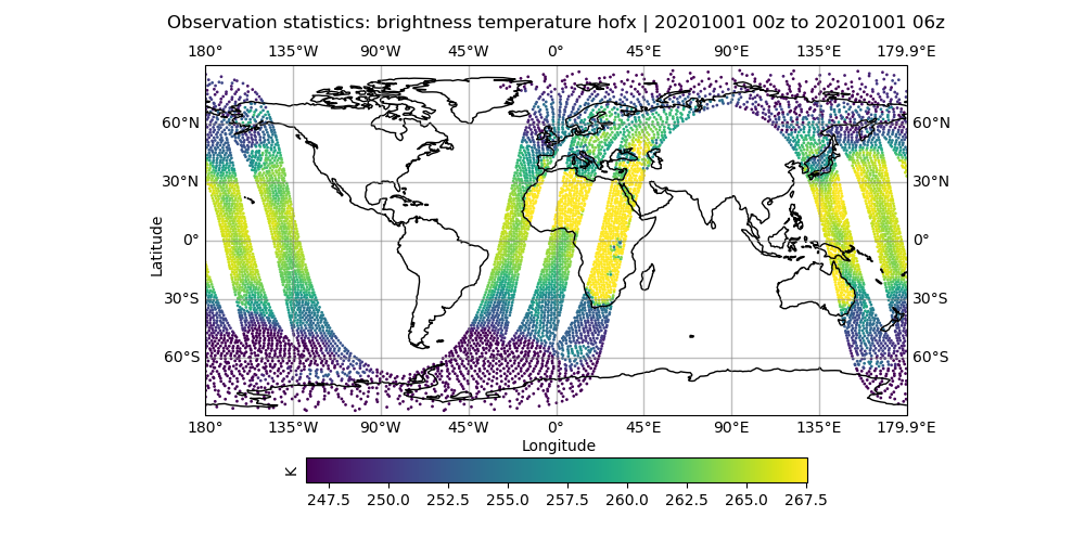
This shows simulated temperature measurements (hofx) over a 6-hour period computed by means of the \(H({\bf x})\) operation described above. Each band of points corresponds to an orbit of the spacecraft. This forward operator relies on JCSDA’s Community Radiative Transfer Model (CRTM) to predict what this instrument would see for that model background state.
This is the default field to plot. But, you can also plot other fields. For example, one thing we may wish to do is to compare the simulated observations, hofx, with the actual observations. To do this, first edit the plot configuration file, config/Amsua_n19_gfs.hofx3d.plot.yaml and look for section like this:
# Group to plot (or omb)
metric: hofx

# Variable to plot
field: brightness_temperature

# Channel to plot
channel: 4
To plot the actual observations, replace “hofx” in the “Group to plot” with ObsValue (capitalization is important):
# Group to plot (or omb)
metric: ObsValue
Now return to the main directory of the tutorial and run the fv3jeditools program as follows:
cd $HOME/jedi/tutorials/Hofx
fv3jeditools.x 2020-10-01T03:00:00 config/Amsua_n19_gfs.hofx3d.plot.yaml
and view the file in the last line of the output:
feh output/plots/Amsua_n19/brightness_temperature-channel4_hofx_20201001_030000.png
You may wish to download the files to your computer or open another remote window to view the two images side by side. Another way to compare them is to edit the configuration file again and change the metric value to omb. This stands for “observation minus background”; the difference between the other two images. Then run the fv3jeditools.x command again to generate the plot.
In data assimilation this is often referred to as the innovation and it plays a critical role in the forecasting process; it contains newly available information from the latest observations that can be used to improve the next forecast.
If you are curious, you can find the application output in the directory called output/hofx. There you’ll see 12 files generated, one for each of the 12 MPI tasks. This is the data from which the plots are created. The output filenames include information about the application (hofx3d), the model and resolution of the background (gfs_c48), the file format (ncdiag), the instrument (amsua), and the time stamp.
Step 4: Explore
The main objective here is to return to Steps 2 and 3 and repeat for different observation types. Try running a different instrument from the list and look at the results in the output/plots directory. As with the Amsua_n19 example, the default plot is hofx but you can edit the configuration file to plot ObsValue or omb instead. Be sure to run the fv3jeditools.x program again to generate a new plot, for example:
fv3jeditools.x 2020-10-01T03:00:00 config/Radiosonde_gfs.hofx3d.plot.yaml
The first argument (the date/time) is the same for all; you just select the configuration file you want. But, be sure to run the run.bash script first to generate the data to plot.
You can also select a different variable to plot by changing the field. Or, for radiance data, you can select the spectral channel. You can determine possible values for these fields by looking in the corresponding jedi configuration file for the run. For example, in the config/Radiosonde_gfs.hofx3d.jedi.yaml file, you’ll find a section like this:
observations:
- obs space:
    name: Radiosonde
    obsdatain:
      obsfile: input/obs/ioda_ncdiag_radiosonde_PT6H_20201001_0300Z.nc4
    obsdataout:
      obsfile: output/hofx/hofx3d_gfs_c48_ncdiag_radiosonde_PT6H_20201001_0300Z.nc4
    simulated variables:
    - eastward_wind
    - northward_wind
    - air_temperature
  obs operator:
    name: VertInterp
This tells you that possible field (variable) values are eastward_wind, northward_wind, and air_temperature.
Note
For those who are familiar with it, running the NetCDF utility ncdump on the output/hofx file is another way to see the fields that are available to plot.
A few suggestions: look at how the aircraft observations trace popular flight routes; look at the mean vertical temperature and wind profiles as determined from radiosondes; discover what observational quantities are derived from Global Navigation Satellite System radio occultation measurements (GNSSRO); revel in the 22 wavelength channels of the Advanced Technology Microwave Sounder (ATMS). For more information on any of these instruments, consult JCSDA’s NRT Observation Modeling web site.