Tutorial: Simulating Observations like JCSDA Near-Real-Time Application
- Learning Goals:
Create simulated observations similar to those highlighted on JCSDA’s Near Real-Time (NRT) Observation Modeling web site
Acquaint yourself with the rich variety of observation operators now available in UFO
- Prerequisites:
Overview
The comparison between observations and forecasts is an essential component of any data assimilation (DA) system and is critical for accurate Earth System Prediction. It is common practice to do this comparison in observation space. In JEDI, this is done by the Unified Forward Operator (UFO). Thus, the principle job of UFO is to start from a model background state and to then simulate what that state would look like from the perspective of different observational instruments and measurements.
In the data assimilation literature, this procedure is often represented by the expression \(H({\bf x})\). Here \({\bf x}\) represents prognostic variables on the model grid, typically obtained from a forecast, and \(H\) represents the observation operator that generates simulated observations from that model state. The sophistication of observation operators varies widely, from in situ measurements where it may just involve interpolation and possibly a change of variables (e.g. radiosondes), to remote sensing measurements that require physical modeling to produce a meaningful result (e.g. radiance, GNSSRO).
So, in this tutorial, we will be running an application called \(H({\bf x})\), which is often denoted in program and function names as Hofx. This in turn will highlight the capabilities of JEDI’s Unified Forward Operator (UFO).
The goal is to create plots comparable to JCSDA’s Near Real-Time (NRT) Observation Modeling web site. This site regularly ingests observation data for the complete set of operational instruments at NOAA. And, it compares these observations to forecasts made through NOAA’s operational Global Forecasting System (FV3-GFS) and NASA’s Goddard Earth Observing System (FV3-GEOS).
But there is a caveat. The NRT web site regularly simulates millions of observations using model backgrounds with operational resolution - and it does this every six hours! That requires substantial high-performance computing (HPC) resources. We want to mimic this procedure in a way that can be run on a laptop computer. So, the model background you will use will be at a much lower horizontal resolution (c48, corresponding to about 14 thousand points in latitude and longitude) than the NRT website (GFS operational resolution of c768, corresponding to about 3.5 million points).
Step 1: Setup
Now that you have finished the Run JEDI in a Container tutorial, you have a containerized version of fv3-bundle ready to go. So, if you are not there already, re-enter the container:
singularity shell -e jedi-tutorial_latest.sif
Now, the description in the previous section gives us a good idea of what we need to run \(H({\bf x})\). First, we need \({\bf x}\) - the model state. In this tutorial we will use background states from the FV3-GFS model with a resolution of c48, as mentioned above.
Next, we need observations to compare our forecast to. Example observations available in this tutorial include (see the NRT website for an explanation of acronyms):
Aircraft
Sonde
Satwinds
Scatwinds
Vadwind
Windprof
SST
Ship
Surface
cris-npp
cris-n20
airs-aqua
gome-metopa
gome-metopb
sbuv2-n19
amsua-aqua
amsua-n15
Amsua-n18
amsua-n19
amsua-metopa
amsua-metopb
amsua-metopc
iasi-metopa
iasi-metopb
seviri-m08
seviri-m11
mhs-metopa
mhs-metopb
mhs-metopc
mhs-n19
ssmis-f17
ssmis-f18
atms-n20
The script to get these background and observation files is in the container. But, before we run it, we should find a good place to run our application. The fv3-bundle directory is inside the container and thus read-only, so that will not do.
So, you’ll need to copy the files you need over to your home directory that is dedicated to running the tutorial:
mkdir -p $HOME/jedi/tutorials
cp -r /opt/jedi/fv3-bundle/tutorials/Hofx $HOME/jedi/tutorials
cd $HOME/jedi/tutorials/Hofx
chmod a+x run.bash
We’ll call $HOME/jedi/tutorials/Hofx the run directory.
Now we are ready to run the script to obtain the input data (from the run directory):
./get_input.bash
You only need to run this once. It will retrieve the background and observation files from a remote server and place them in a directory called input.
You may have already noticed that there is another directory in your run directory called config. Take a look. Here are a different type of input files, including configuration (yaml) files that specify the parameters for the JEDI applications we’ll run and fortran namelist files that specify configuration details specific to the FV3-GFS model.
Step 2: Run the Hofx application
There is a file in the run directory called run.bash. Take a look. This is what we will be using to run our Hofx application.
When you are ready, try it out:
./run.bash
If you omit the arguments, the script just gives you a list of instruments that are available in this tutorial. For Step 2 we will focus on radiance data from the AMSU-A instrument on the NOAA-19 satellite:
./run.bash Amsua_n19
Skim the text output as it is flowing by. Can you spot where the quality control (QC) on the observations is being applied?
Step 3: View the Simulated Observations
You’ll find the graphical output from Step 2 in the output/plots/Amsua_n19 directory.
You can use the linux utility feh to view the png files:
cd output/plots/Amsua_n19
feh brightness_temperature_12_ObsValue.png
If you get an error message it may be because you are accessing singularity from a remote machine. As with other remote graphical applications, you need to make sure you use the -Y option to ssh to enable X forwarding, e.g. ssh -Y .... Another tip is to open another window on that same machine and see what your DISPLAY environment variable is set to:
echo $DISPLAY # run this from outside the container
Then, set the DISPLAY variable to be the same inside the container, for example:
export DISPLAY=localhost:11.0
If this still does not work, it might be worthwhile to copy the png files to your laptop or workstation for easier viewing. Similar arguments apply if you are running singularity in a Vagrant virtual machine: see our Vagrant documentation for tips on setting up X forwarding in that case or on viewing the files from the host.
When are able to view the plot, it should look something like what is shown on the JCSDA NRT web site:
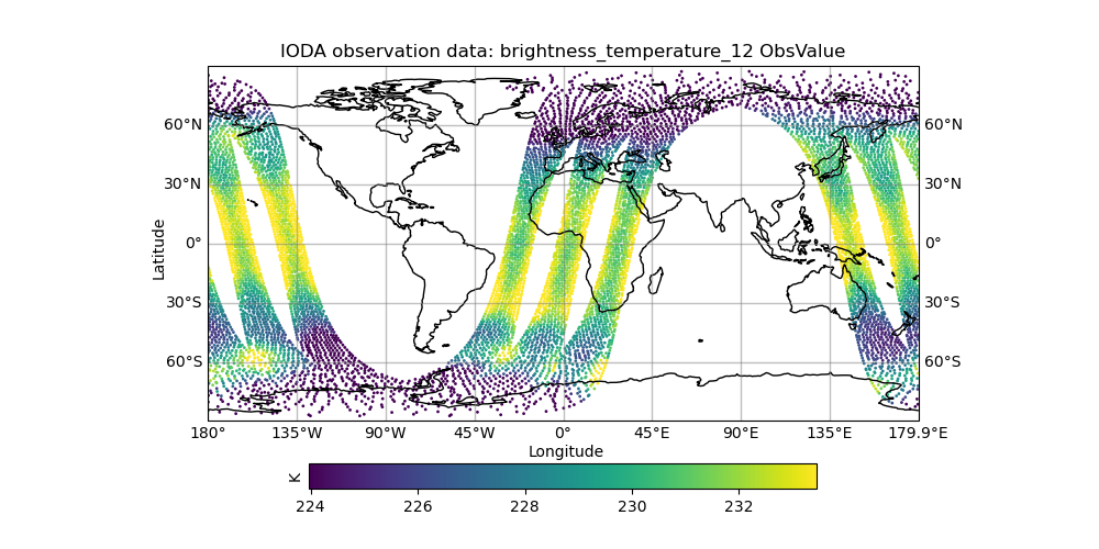
This shows temperature measurements over a 6-hour period. Each band of points corresponds to an orbit of the spacecraft.
Now look at some of the other fields. The files marked with ObsValue correspond to the observations and the files marked with hofx represent the simulated observations computed by means of the \(H({\bf x})\) operation described above. This forward operator relies on JCSDA’s Community Radiative Transfer Model (CRTM) to predict what this instrument would see for that model background state.
The files marked omb represent the difference between the two: observations minus background. In data assimilation this is often referred to as the innovation and it plays a critical role in the forecasting process; it contains newly available information from the latest observations that can be used to improve the next forecast. To see the innovation for this instrument over this time period, view this file:
feh brightness_temperature_12_latlon_ombg_mean.png
If you are curious, you can find the application output in the directory called output/hofx. There you’ll see 12 files generated, one for each of the 12 MPI tasks. This is the data from which the plots are created. The output filenames include information about the application (hofx3d), the model and resolution of the background (gfs_c48), the file format (ncdiag), the instrument (amsua), and the time stamp.
Step 4: Explore
The main objective here is to return to Steps 2 and 3 and repeat for different observation types. Try running another observation type and look at the results in the output/plots directory. A few suggestions: look at how the aircraft observations trace popular flight routes; look at the mean vertical temperature and wind profiles as determined from radiosondes; discover what observational quantities are derived from Global Navigation Satellite System radio occultation measurements (GNSSRO); revel in the 22 wavelength channels of the Advanced Technology Microwave Sounder (ATMS). For more information on any of these instruments, consult JCSDA’s NRT Observation Modeling web site.
The most attentive users may notice an unused configuration file in the config directory called Medley_gfs.hofx3d.jedi.yaml. Advanced users may seek to run this themselves, guided by the run.bash script. This runs a large number of different observation types so it takes much longer to run. This is included in the tutorial merely to give you the flavor of what is involved in creating the NRT site. This generates plots for over 40 instruments every six hours, using higher-resolution model backgrounds that have more than 250 times more horizontal points than what we are running here. The GEOS-NRT site goes a step further in terms of computational resources - displaying continuous 4D \(H({\bf x})\) calculations.