Explicit Diffusion

The Explicit Diffusion block uses a forward stepping finite-difference method to propagate background error covariances by numerically solving the explicit diffusion equation. In one dimension, the diffusion equation is:

\[u_i^{n+1} = u_i^n + k \dfrac{(u_{i+1}^n -2u_i^n + u^n_{i-1})}{\Delta x^2} \Delta t\]

where \(u^i\) represents the analysis increment at grid index \(i\). The iteration index \(n\) represents a step in propagating the covariance across the grid, and though it is related to \(\Delta t\), neither of these quantities represent an actual time (measured in seconds or hours). \(k\) is the diffusion constant which (along with \(\Delta t\)) sets how ‘quickly’ an impulse from observations will propagate to nearby grid points.

On a 1D grid with \(N\) points, there is one diffusion equation for each grid point resulting in a system of \(N\) equations which can be easily translated into a sparse matrix equation – with the signature 3-point, 1D laplacian stencil element \([..., 0, 1, -2, 1, 0, ...]\) along the diagonal – and directly solved. In 2D, a 9-point stencil is typically used:

\[\begin{split}\begin{vmatrix} 0 & 1 & 0\\ 1 & -4 & 1\\ 0 & 1 & 0 \end{vmatrix}\end{split}\]

There is physical significance in how the values in the stencil elements sum to zero. When a physical substance diffuses, more substance is not created nor is the substance destroyed. In the 1D case, the stencil is reflecting the diffusive property that 2 units of the substance leaves a point \(i\) and one unit moves left (to point \(i-1\)) and the other unit moves right (to the point \(i+1\)). If the initial concentration of the substance has a peak value of 1, then this peak will decrease as the substance diffuses. This conservation property does not apply with the application of a B matrix on an analysis increment. In background error modeling, the correlation (corresponding to the concentration in the physical analogy) should have a peak at 1, since the peak of the error correlation within the B matrix occurs along the diagonal, representing the error correlation of a grid point with itself.

To keep the peak error correlation at a value of 1 throughout the iterative application of the explicit, forward-stepping a calibration factor must be pre-calculated and applied at each iteration.

For a simple example, consider how a gaussian shaped impulse is propagated by a diffusion operator:

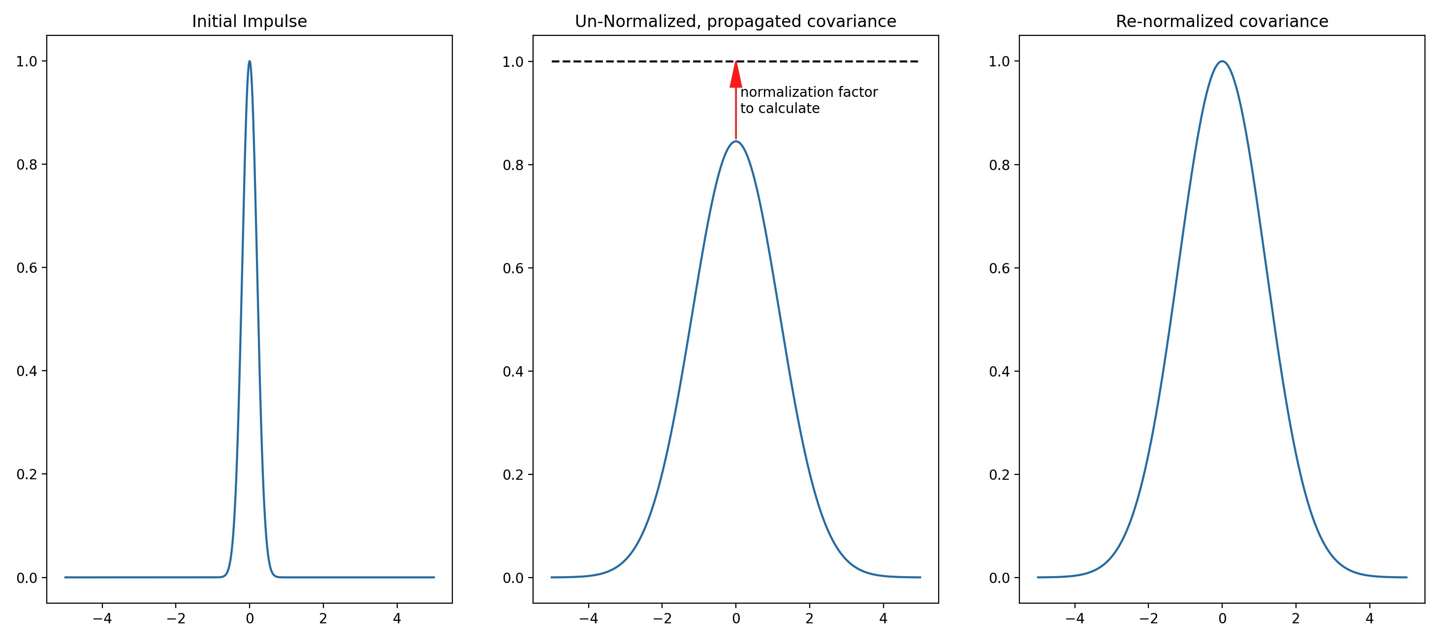
Fig. 9 Illustration of the calibration process for the Explicit Diffusion block in 1D. The curves on the left and in the middle of this illustration have not been drawn to scale in order to more clearly demonstrate the process. In a real case, the areas under the curves on the left and in the middle are equal.

Calibration Method

Many SABER blocks, especially central blocks, require a calibration process for tuning the block to the specific case in which it will be used. The calibration for the Explicit Diffusion block has factored the process into a horizontal (2D) part and a vertical (1D) part. In total, the two parts determine the normalization needed to maintain the peak correlation as close to 1 as possible, for each grid point, through the iterative application of the diffusion operator when the block is applied as part of a B matrix.

The horizontal normalization process uses a ‘randomization method’ (as described in [WCMP21]) which is related to, but distinct from, the randomization mode of The ErrorCovarianceToolbox Application. Both refer to the process of applying the square root of the B matrix to a vector of random perturbations to produce an ensemble member. The randomization method for calibrating the Explicit Diffusion normalization uses the SABER randomization procedure. The calibration process iteratively produces a state (utilizing the SABER randomization), applies the forward diffusion operator, and updates a set of statistics. The number of iterations is set by the user in the application’s configuration (see the example in Calibration Example). After all the iterations are completed, the final set of normalization coefficients are calculated and written out to a file.

This horizontal calibration can occur off-line and is grid-specific, so the file produced can be reused in new applications as long as the B matrix grid does not change.

The vertical normalization process is more straight forward and faster computationally since it takes advantage of how vertical columns of points in an atlas::Field are entirely owned by a single PE. To determine the vertical normalization, the full B matrix is applied to a dirac ‘sheet’ (a state with 1’s at all points on a single level and 0’s on all other levels) for each level, and a normalization value is calculated for each column.

For covariance modeling in the ocean (where vertical structure, e.g. the vertical location of the thermocline, can change on short time scales), this vertical normalization typically occurs on-line at each DA cycle.

Practical considerations

The ratio of \(\dfrac{k\Delta t}{\Delta x^2}\) encodes the CFL condition: a trade off between the stability of the method and how quickly it will run. If the ratio is too large (i.e. \(k \Delta t \gtrsim {\Delta x^2}\)), the method will be unstable and produce an unphysical representation of background errors. This value is not set by a user, instead the Explicit Diffusion block calculates a value for \(k \Delta t\) that satisfied the CFL condition based on the smallest grid spacing of the B matrix grid geometry.

This instability associated with large values of \(\Delta t\) is a practical reason the Explicit Diffusion block is better for modeling short-scale background error covariances: it would take too many iterations to ‘diffuse’ the long-scale errors.

Also, the matrix form of the finite difference diffusion equation makes it relatively simple to apply complex boundary conditions, like a land mask. This makes diffusion an advantageous method for modeling background errors in the ocean.

YAML configurations

Calibration Example

The calibration (error covariance training) mode calculates the normalizations which keeps the ‘peak’ correlation at 1 (instead of decreasing to a lower value), and writes the normalization coefficients to a file. The length scale for the covariance (either the localization length if used as an ensemble B, or the correlation length if used as a static B), is set in the calibration step.

To set the localization length(s), users have the option to set a single, global value using the fixed value: key, or users can read in a model file to set a location-dependent localization scale. These options are demonstrated, respectively, in the horizontal configuration and vertical configuration in the example below:

saber central block:
  saber block name: diffusion
  calibration:
    normalization:
      iterations: 1000 #sets the number of calibration iterations
    groups:
    - horizontal:
        fixed value: 3000.0e3 #sets the localization length scale (in meters)
      write:
        filepath: <path/to/data>/<horizontal_normalization_filename>
    - vertical:
        model file:
          ... # configuration for reading a model file
        levels: <num_levels> # MUST MATCH the number of levels in model
        as gaussian: true
      write:
        filepath: <path/to/data>/<vertical_normalization_filename>

A recommended number of normalization iterations (which only applies to the horizontal calibration) for an operational configuration is 20,000. This value is independent of the grid size/resolution. Ideally, this value is as large as computationally feasible/practical.

Variational Example

After calibration, when using the block to apply background errors to an analysis increment, simply point to the files produced by the calibration step. The number of iterations required to reach the length scale set in the calibration is pre-calculated by the block.

saber central block:
saber block name: diffusion
read:
  groups:
  - variables: *vars
    horizontal:
      filepath: <path/to/data>/<horizontal_normalization_filename>
    vertical:
      levels: *levels
      filepath: <path/to/data>/<vertical_normalization_filename>

More Information

Deeper descriptions of how the calibration procedure and horizontal/vertical splitting are implemented in SABER are available in the reference below (note, the reference discusses implicit diffusion, but the splitting and calibration procedures are implemented in the Explicit Diffusion block as described in the paper):

Weaver AT, Chrust M, Ménétrier B, Piacentini A. An evaluation of methods for normalizing diffusion-based covariance operators in variational data assimilation. Q J R Meteorol Soc. 2021; 147: 289–320. https://doi.org/10.1002/qj.3918