IODA Interfaces
Background
In the context of running a DA flow, IODA interacts with external observation data on one side and with the OOPS and UFO components of JEDI on the other side (Fig. 5). On the observation data side there exist huge amounts of data, thus creating the need to pare these data down to a manageable size for JEDI during a particular DA run. The primary mechanism for accomplishing this is to filter out all of the observations that lie outside the current DA timing window, and present only that subset to be read into memory during a DA run.
There are many different types of observations that come with a variety of ways that the observation data are organized. To the extent that is feasible, it is desirable to devise a common data organization of which all of these observation types can employ. This is where the IODA Data Model (Fig. 6) comes into play. The IODA Data Model provides a means for storing conventional (1D trajectories) and radiance (2D images) data in a common Group, Variable and Attribute structure.
A schematic representation of the IODA data model is shown in (Fig. 12).
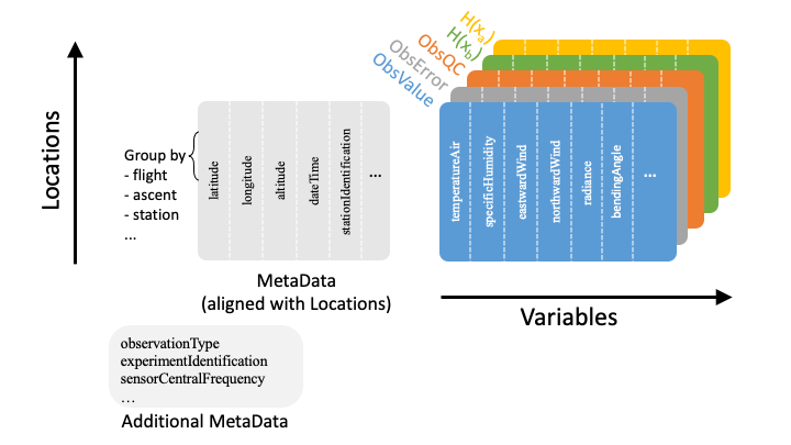
Fig. 12 Schematic representation of the IODA data model
Central to this scheme are the 2D tables holding the observation data quantities (ObsValue, ObsError, HofX in Fig. 12). Note that a given Group (ObsValue, MetaData, etc.) in the IODA Data Model represents a particular table in the schematic, and the Variables contained by that group are represented by the columns of the associated table. Each column of a given table holds a particular variable of observation data, where each variable can be a vector (1D), matrix (2D) or of higher rank. The height of each column is equal to the number of unique locations, (x,y,z,t) or (x,y,t) tuple values, and the number of columns corresponds to the set of available observation variables. Note that an ObsVector can be constructed using a subset of the variables (columns) in a given table.
In addition to the primary data tables (Fig. 12, color), tables of meta data (Fig. 12, gray) can be stored. The MetaData table (related to locations) contains columns (variables) corresponding to meta data associated with each location. Examples of location-related meta data are quantities that describe each location such as Latitude, Longitude, Date/Time, and descriptive quantities associated with locations such the Scan Angle of a satellite-borne instrument.
The Additional MetaData table is similar to the MetaData array, except that it holds meta data associated with other dimensions than the locations dimension. Examples include the variable names, and in the case of satellite instruments, channel frequencies.
A primary design principle for IODA is to not alter the original observations and meta data that was received from the data providers. Nervertheless, there are still important fuctions that IODA needs to perform as shown in Fig. 13.
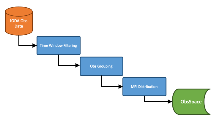
Fig. 13 Operations performed by IODA when reading in observation data
IODA performs three operations that must go in the order shown in Fig. 13. First all observations that lie outside the DA time window are removed. Then the locations are organized into groups called “records” according to optional specifications that can be entered in the YAML configuration. The default is to place each individual location into its own unique record (no grouping). An example is to organize radiosonde locations by station ID and launch time (ie, locations with matching station ID and launch time values are grouped together into a single record) so that records contain individual soundings. Lastly the records are distributed to MPI tasks according to distribution specifications in the YAML configuration. The point of doing the observation grouping before the MPI distribution is to ensure that IODA does not break up the groups (e.g., radiosonde soundings) during the MPI distribution step.
IODA also handles the transfer of observation data between the GTS network (data providers) and the diagnostics/monitoring system (Fig. 3). As of the JEDI 1.1.0 release, the IODA architecture (Fig. 4) is targeted to handle these tasks and work is actively progressing to migrate the current implementaions (e.g. ioda converters, diagnostic plotting tools) to the IODA client API.
Example Radiosonde YAML
The following is a YAML example for configuring the processing of radiosonde data in UFO.
window begin: 2018-04-14T21:00:00Z
window end: 2018-04-15T03:00:00Z
observations:
- obs space:
    name: Radiosonde
    obsdatain:
      obsfile: Data/testinput_tier_1/sondes_obs_2018041500_m.nc4
      obsgrouping:
        group variables: [ "station_id" ]
        sort variable: "air_pressure"
        sort order: "descending"
    obsdataout:
      obsfile: Data/sondes_obs_2018041500_m_out.nc4
    simulated variables: [air_temperature]
  obs operator:
    name: VertInterp
    vertical coordinate: air_pressure
  geovals:
    filename: Data/sondes_geoval_2018041500_m.nc4
  vector ref: GsiHofX
  tolerance: 1.0e-04  # in % so that corresponds to 10^-3
  linear obs operator test:
    iterations TL: 12
    tolerance TL: 1.0e-9
    tolerance AD: 1.0e-11
The obs space.obsdatain.obsgrouping keyword is used to initate the obs grouping step in the IODA input flow (Fig. 13).
This specification is requesting that IODA group locations according the MetaData variable “station_id” (“MetaData/station_id”).
All locations with the same unique station_id value will be grouped into an individual record
before doing the MPI distribution step.
The intent of this specification is to keep individual soundings intact during the MPI distribution step.
It is possible to define more than one grouping variable if that is necessary to uniquely identify records in the data set.
The observations will be grouped according to the first variable in the list, then each group will be divided further according to the second variable, etc.
IODA has an additional feature that provides functions that denote the sorting of locations within each record.
A MetaData variable and sort order is specified to enable and drive this feature.
The obs space.obsdatain.obsgrouping.sort variable and obs space.obsdatain.obsgrouping.sort order are telling IODA to use the values of the “MetaData/air_pressure” variable in corresponding locations to sort the soundings into ascending order (i.e., descending pressure values).
Under the obs space.obsdataout.obsfile specification, the output file is requested to be created in the path: Data/sondes_obs_2018041500_m_out.nc4.
IODA tags the MPI rank number onto the end of the file name (before the “.nc4” suffix) so that multiple MPI tasks writing files do not collide.
If there are 4 MPI tasks, then the output will appear in the following four files:
Data/sondes_obs_2018041500_m_out_0000.nc4
Data/sondes_obs_2018041500_m_out_0001.nc4
Data/sondes_obs_2018041500_m_out_0002.nc4
Data/sondes_obs_2018041500_m_out_0003.nc4
More details about constructing and processing YAML configuration files can be found in JEDI Configuration Files: Content and Configuring JEDI.
Interfaces to other JEDI Components
For the JEDI 1.1.0 release, the ObsSpace and ObsVector interfaces remained backward compatible with the existing OOPS and UFO facing interfaces which are described below. After the release, the stage will be set to migrate the relevant classes to directly utilize the IODA client API (Fig. 4). Once accomplished the OOPS and UFO interfaces below will be obsoleted and replaced with the much richer IODA client API. See the low-level description of the classes, functions, and subroutines for details about the client API.
OOPS Interface
OOPS accesses observation data via C++ methods belonging to the ObsVector class.
The variables being assimilated are selected in the YAML configuration using the simulated variables sub-keyword under the obs space keyword.
In the radiosonde example above, one variable “air_temperature” is being assimilated.
In this case, the ObsVector will read only the air_temperature row from the ObsSpace and load that into a vector.
The ObsVector class contains the following two methods, read() for filling a vector from an ObsSpace in memory and save() for storing a vector into an ObsSpace.
// Interface prototypes
void read(const std::string &);
void save(const std::string &) const;
The
std::stringarguments are the names of the ObsSpace Group that is to be accessed.
Following is an example of reading into an observation vector.
Note that the ObsVector object yobs_ has already been constructed which included the allocation of the memory to store the observation data coming from the read() method.
// Read observation values
Log::trace() << "CostJo::CostJo start" << std::endl;
yobs_.read("ObsValue");
Log::trace() << "CostJo::CostJo done" << std::endl;
Here is an example of saving the contents of an observation vector, H(x), into an ObsSpace. The ObsVector object yobs is constructed in the first line, and the third line creates an ObsSpace Group called “hofx” and stores the vector data into that ObsSpace.
//  Save H(x)
boost::scoped_ptr<Observations_> yobs(pobs->release());
Log::test() << "H(x): " << *yobs << std::endl;
yobs->save("hofx");
UFO Interface
UFO accesses observation data via Fortran functions and subroutines belonging to the ObsSpace class. ObsSpace is implemented in C++ and a Fortran interface layer is provided for UFO. The following three routines are used to access observation data, and unlike the ObsVector methods in the OOPS Interface above, access is available to ObsSpace Groups and all MetaData variables. Reasons to access ObsSpace Groups from UFO would be for debugging purposes or for storing results, such as H(x), for post analysis. Typically, only meta data are used in the actual H(x) calculations.
! Interface prototypes
integer function obsspace_get_nlocs(obss)
subroutine obsspace_get_db(obss, group, vname, vect)
subroutine obsspace_put_db(obss, group, vname, vect)
The
obssarguments are C pointers to ObsSpace objects.- The
grouparguments are names of the ObsSpace Group holding the requested variable E.g., “HofX”, “MetaData”
- The
- The
vnamearguments are names of the requested variable (column) E.g., “air_temperature”, “Scan_Angle”
- The
- The
vectargument is a Fortran array for holding the data values The client (caller) is responsible for allocating the memory for the
vectargument
- The
Following is an example from the CRTM radiance simulator, where meta data from the instrument are required for doing the simulation.
! Get nlocs and allocate storage
nlocs = obsspace_get_nlocs(obss)
allocate(TmpVar(nlocs))

! Read in satellite meta data and transfer to geo structure
call obsspace_get_db(obss, "MetaData", "Sat_Zenith_Angle", TmpVar)
geo(:)%Sensor_Zenith_Angle = TmpVar(:)

call obsspace_get_db(obss, "MetaData", "Sol_Zenith_Angle", TmpVar)
geo(:)%Source_Zenith_Angle = TmpVar(:)

call obsspace_get_db(obss, "MetaData", "Sat_Azimuth_Angle", TmpVar)
geo(:)%Sensor_Azimuth_Angle = TmpVar(:)

call obsspace_get_db(obss, "MetaData", "Sol_Azimuth_Angle", TmpVar)
geo(:)%Source_Azimuth_Angle = TmpVar(:)

call obsspace_get_db(obss, "MetaData", "Scan_Position", TmpVar)
geo(:)%Ifov = TmpVar(:)

call obsspace_get_db(obss, "MetaData", "Scan_Angle", TmpVar) !The Sensor_Scan_Angle is optional
geo(:)%Sensor_Scan_Angle = TmpVar(:)

deallocate(TmpVar)
An example for storing the results of a QC background check is shown below. Note that the storage for “flags” has been allocated and “flags” has been filled with the background check results prior to this code.
write(buf,*)'UFO Background Check: ',ireject,trim(var),' rejected out of ',icount,' (',iloc,' total)'
call fckit_log%info(buf)

! Save the QC flag values
call obsspace_put_db(self%obsdb, self%qcname, var, flags)