Goals and code organization
Scientific goals
Background error covariance modelling is a key feature of data assimilation systems. Since geophysical models (atmosphere, ocean, sea-ice, land surface, etc.) use very diverse model grids, structured or unstructured, global or regional, sometimes with complex boundaries, it seems relevant to implement background error covariances on a generic unstructured mesh. The software BUMP (Background error on Unstructured Mesh Package) is precisely designed for this purpose, to diagnose and apply background error covariance related operators efficiently on a generic unstructured mesh.
Three categories of background error covariance models are currently implemented in BUMP:
The ensemble covariance model is built as a transformed and localized sample covariance matrix:
\[\mathbf{B}_e = \mathbf{T} \left(\mathbf{T}^{-1} \widetilde{\mathbf{B}} \mathbf{T}^{-\mathrm{T}} \circ \mathbf{L}\right) \mathbf{T}^\mathrm{T}\]where:
\(\widetilde{\mathbf{B}} \in \mathbb{R}^{n \times n}\) is the sample covariance matrix estimated from an ensemble,
\(\mathbf{T} \in \mathbb{R}^{n \times n}\) is an invertible transformation matrix,
\(\mathbf{L} \in \mathbb{R}^{n \times n}\) is the localization matrix,
\(\circ\) denotes the Schur product (element-by-element).
The static covariance model is build with successive parametrized operators:
\[\mathbf{B}_s = \mathbf{U}_b \boldsymbol{\Sigma} \mathbf{C} \boldsymbol{\Sigma} \mathbf{U}_b^\mathrm{T}\]where:
\(\mathbf{U}_b \in \mathbb{R}^{n \times n}\) is a multivariate balance operator,
\(\boldsymbol{\Sigma} \in \mathbb{R}^{n \times n}\) is a diagonal matrix containing standard deviations,
\(\mathbf{C} \in \mathbb{R}^{n \times n}\) is a block diagonal (univariate) correlation matrix.
The hybrid covariance model is a linear combination of both previous models:
\[\mathbf{B}_h = \beta_e^2 \mathbf{B}_e + \beta_s^2 \mathbf{B}_s\]where \(\beta_e \in \mathbb{R}\) and \(\beta_s \in \mathbb{R}\) are scalar coefficients.
The first step of BUMP is to use an ensemble of forecasts to diagnose \(\mathbf{U}_b\), \(\boldsymbol{\Sigma}\), \(\mathbf{C}\), \(\mathbf{L}\) or \(\mathbf{T}\), and optionally a second ensemble randomized from \(\mathbf{B}_s\) to diagnose \(\beta_e\) and \(\beta_s\). No observation is used in BUMP, only ensembles of forecasts. The second step of BUMP is to apply all these operators efficiently, via simple interfaces.
Code architecture
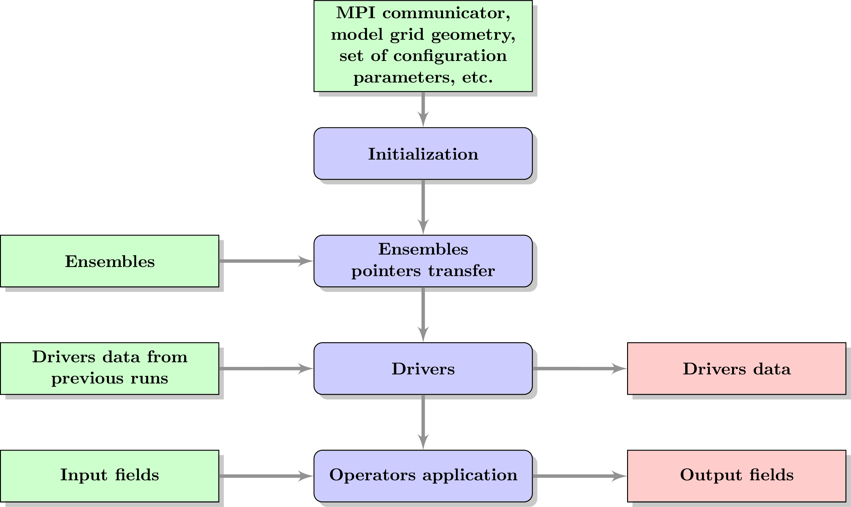
Running BUMP requires four steps: initialization, transferring ensembles pointers, running the drivers, and finally applying BUMP operators.
For the initial setup, BUMP requires various inputs:
MPI communicator,
model grid geometry,
set of configuration parameters,
etc.
Several core features of BUMP are initialized:
parallelization aspects (MPI, OpenMP, parallel I/O),
configuration parameters (consistency checking),
missing values,
output unit for logging,
random number generator,
model and working grids geometry,
masks,
etc.
Ensembles pointers are transferred from the calling code to the BUMP library using an extension of ATLAS fieldsets. The model grid can have redundant points (points with the same longitude/latitude/level), but these points are removed on the internal working grid of BUMP if needed.
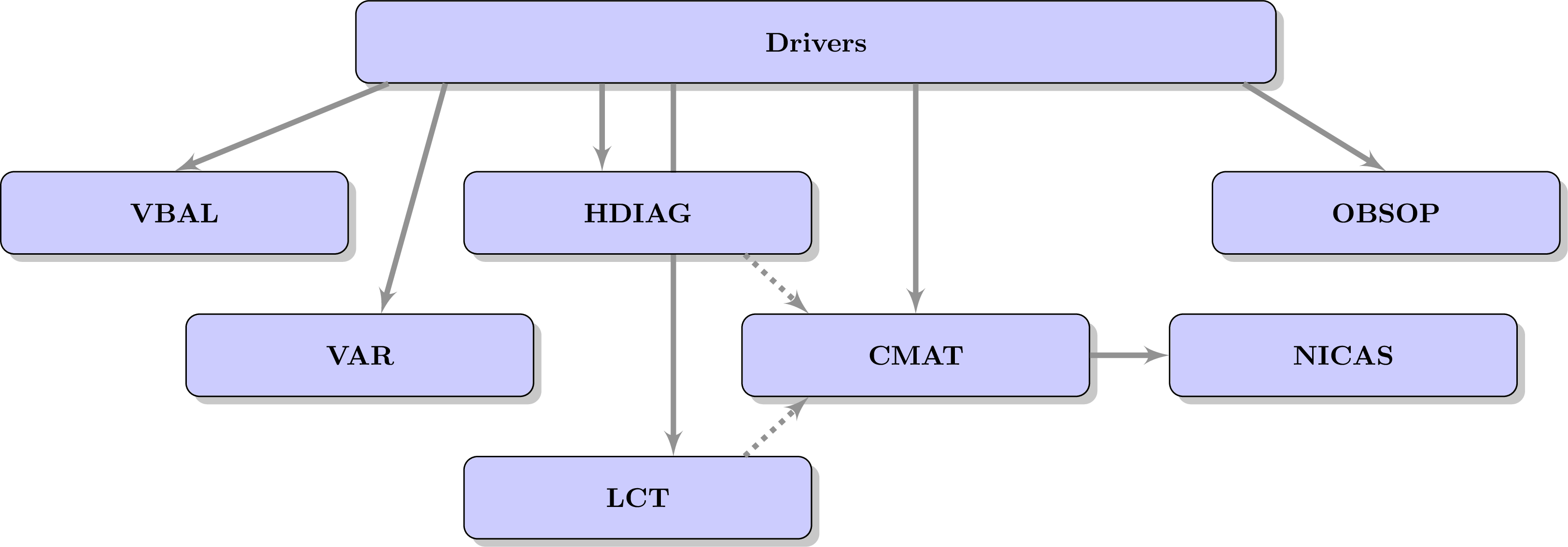
Drivers do the actual jobs required in the configuration parameters. There are different types of drivers, and the order in which they are run can matter:
Dead-end drivers are run first. They implement some diagnostics used for scientific experiments, but their outputs are not used any further in the code.
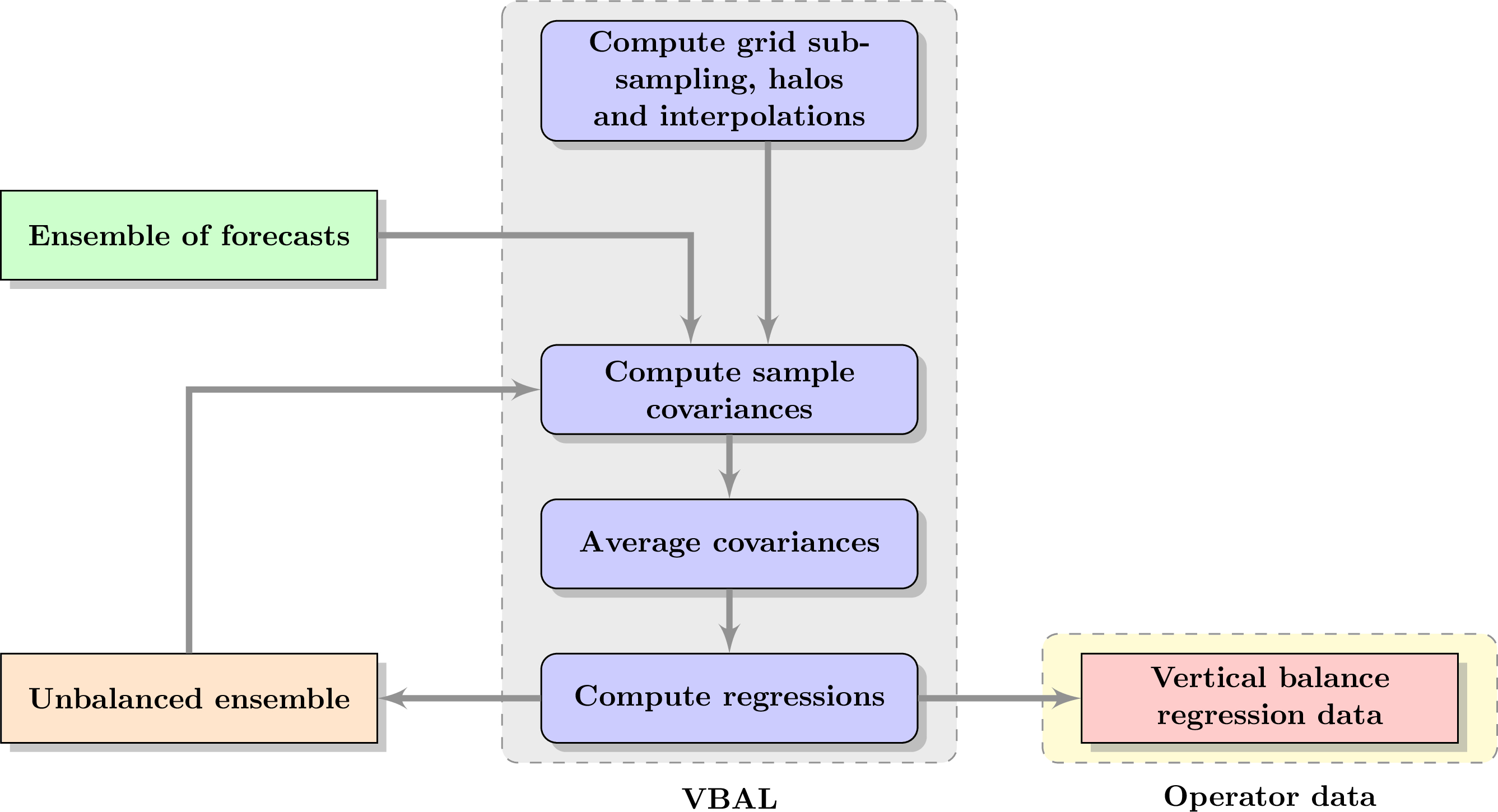
The VBAL driver (for Vertial BALance) computes the vertical balance operator using the first ensemble and writes output data. Data can also be loaded directly. A second driver performs adjoint and inverse tests.
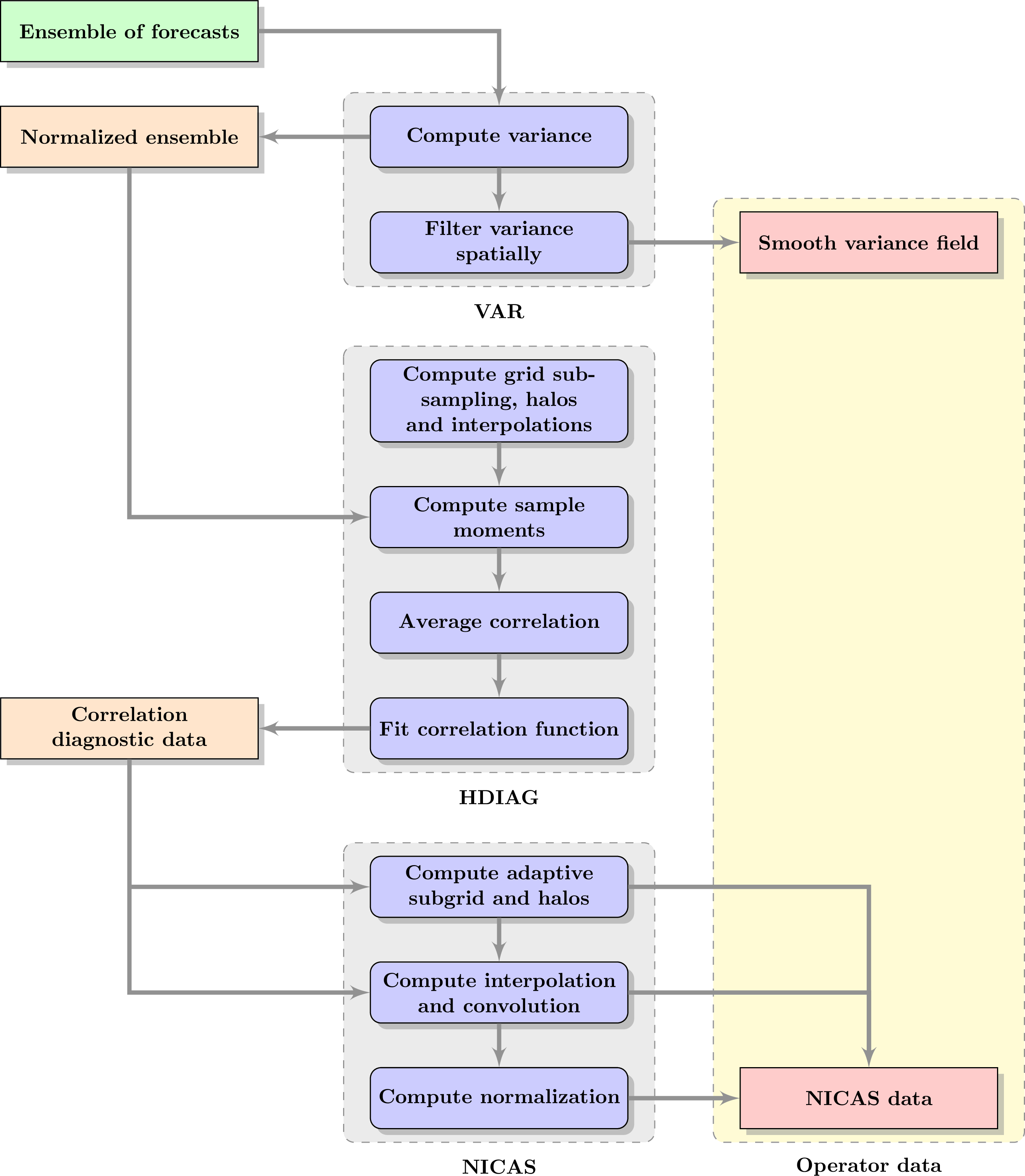
The VAR driver (for VARiance) computes the variance of the ensemble, optionally filters it with an iterative method and writes output data.
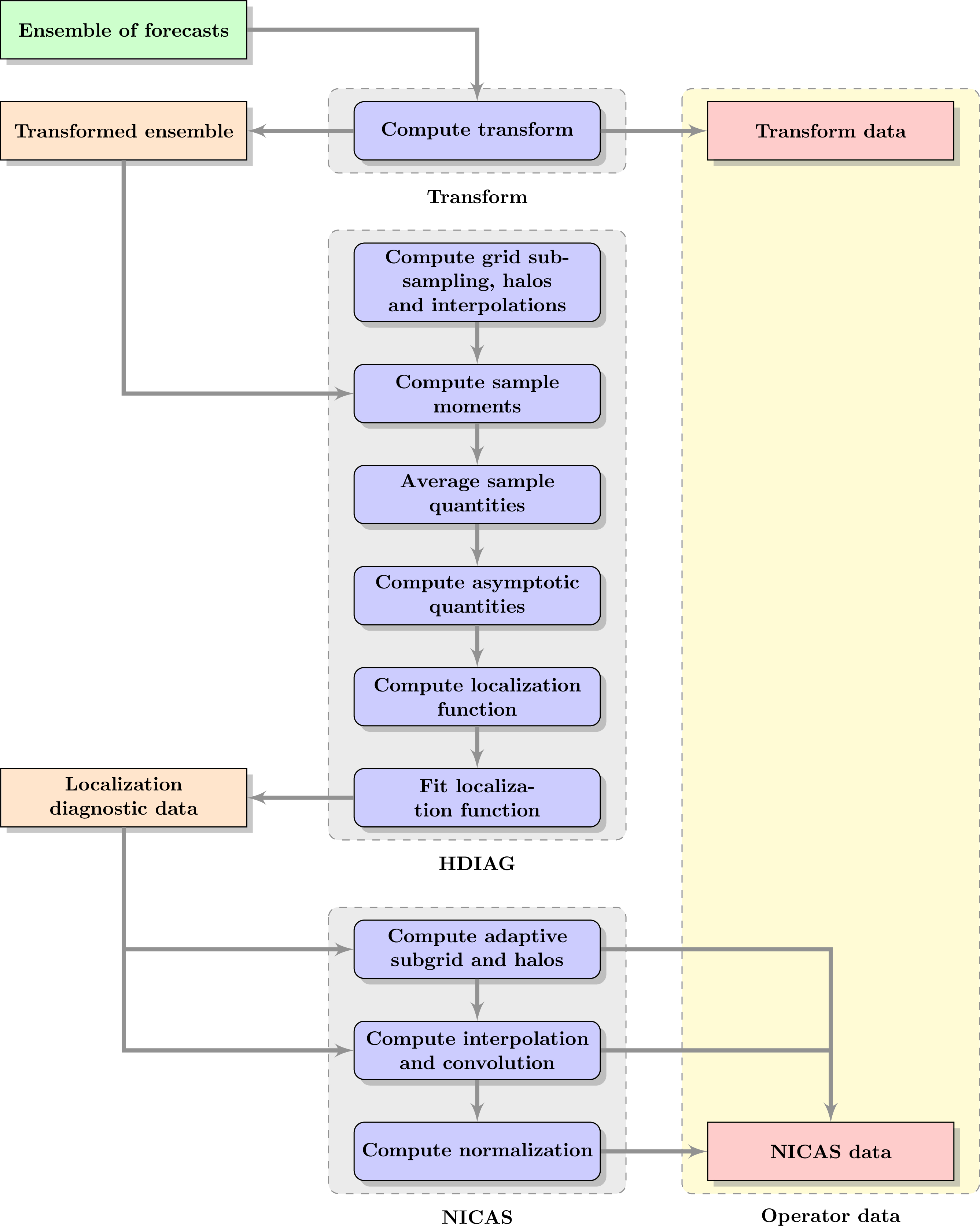
The HDIAG driver (for Hybrid DIAGnostics) computes locally homogeneous and isotropic correlation and localization functions using the first ensemble, determines their length-scales. It also estimates hybrid weights using the second ensemble. Output data are interpolated on the working grid and stored into the CMAT object (for Correlation MATrix).
The LCT driver (for Local Correlation Tensor) computes anisotropic correlation functions and determines the corresponding LCT. Output data are interpolated on the working grid and stored into the CMAT object.
The CMAT fields can also be read from files, modified via the interface, or via configuration parameters. After all the possible modifications, they are written to files again.
The NICAS driver (for Normalized Interpolated Convolution on and Adaptive Subgrid) computes indices and weights for the NICAS smoother using the CMAT data and writes output data. Data can also be loaded directly. A second driver performs various tests (adjoint, Dirac, randomization, consistency, optimality).
The OBSOP driver (for OBServation OPerator) computes interpolation indices and weights given the observations coordinates and writes output data. Data can also be loaded directly. A second driver performs an adjoint test.
Once the drivers have initialized all the BUMP operators, these operators can be applied on data using interfaces:
VBAL operator: direct, inverse, adjoint, inverse adjoint.
VAR operator: direct square-root, inverse square-root.
NICAS operator: full, square-root, square-root adjoint, randomization.
OBSOP operator: direct, adjoint.
Here is a graphical summary of the code architecture:
and the drivers dependencies: